Quantile Regression
The Median Isn’t the Message - Stephen Jay Gould
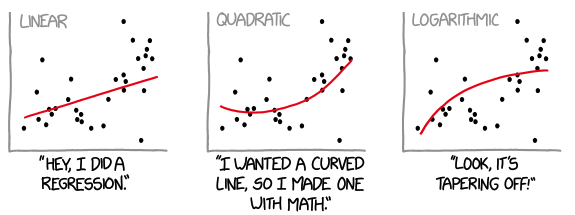
When we think of regression, the most common one, which we all know, is linear regression. It is a fairly popular and simple technique for estimating the mean of some variable conditional on the values of independent variables.
Now imagine if you are a grocery delivery or ride-hailing service and want to show the customer the estimated delivery or wait times. If the distance is smaller, there will be less variability in the waiting time, but if the distance is longer, many things can go wrong, and due to that there can be a lot of variability in the estimate time. If we have to create a model to predict that, we may not want to apply linear regression as that will only tell us the average time.
It’s important to note that one of the key assumptions for applying linear regression is a constant variance (Homoskedasticity). However, many times this is often not the case. The variability is not constant (Heteroscedastic), which violates the linear regression assumption (Linear Regression Notes).
Motivation
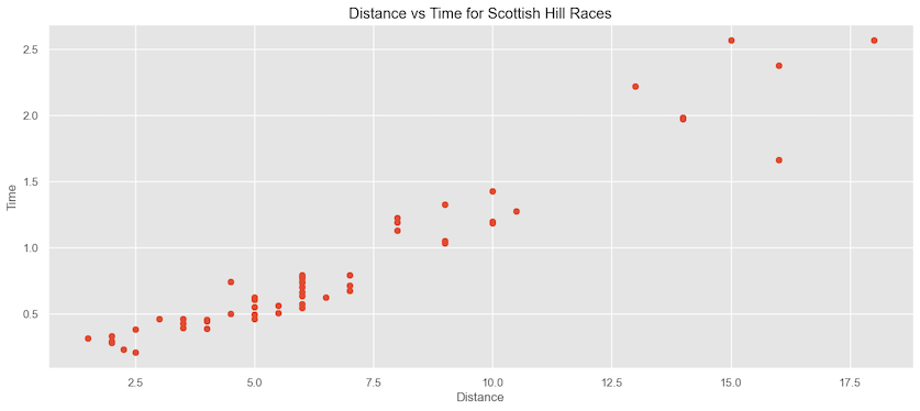
Let’s look at a running data for the distance vs. the time it takes to finish. We clearly know there is a some sort of linear relationship as the distance increases, time to finish also increases.
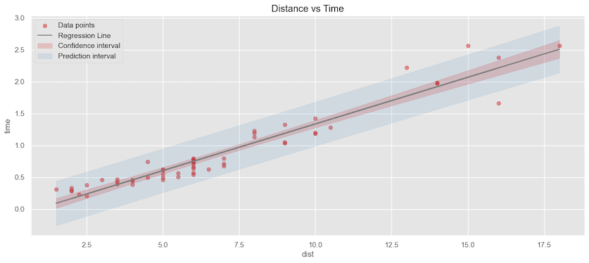
If we apply linear regression and plot the confidence interval of the estimated mean and the prediction intervals. We can see it’s a pretty good fit. Most of the data points are covered in the prediction interval, and given a distance, we can predict the estimated time on an average. The adjusted $R^2=0.921$, which tells the model fits very well.
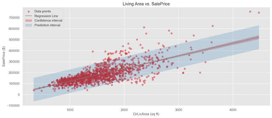
Now, let’s take a look at another dataset and see the relationship between living area and Sale Price. We can see that for lower living areas, the sale price points are very bundled together with little variance; however, as the living area increases, the sale price variation increases a lot.
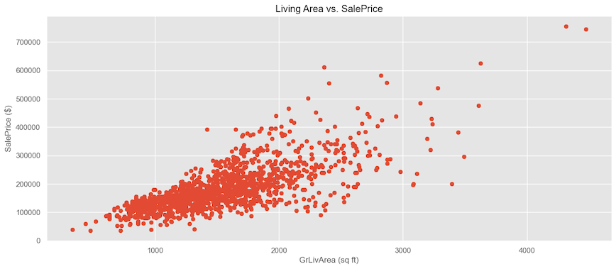
If we apply linear regression and plot the mean and the prediction intervals, we can see how many of the data points are out of the prediction interval. The adjusted $R^2=0.540$, tells that the model doesn’t fit the data very well. For example, if we want to estimate the cost of a house with a living area of 2500 sq. ft., the model predicts the average price is ~300K$. However, if we look at the data, there is a significant variance; the house can go anywhere between 100K and 500K.
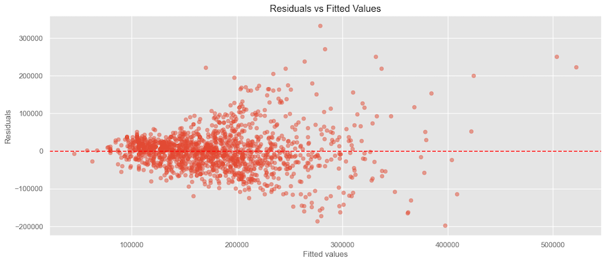
Looking at the residual plot, we can see how the error variation increases, indicating the data is heteroscedastic.
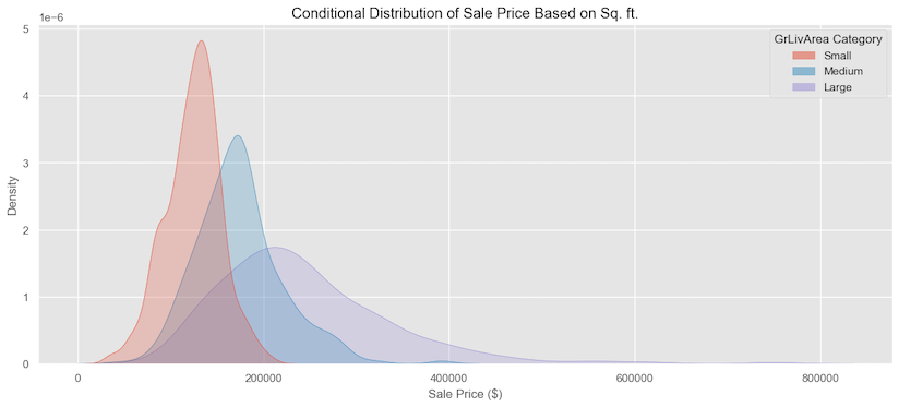
If we break the Living area into three categories: small, medium, and large, such that anything less than 1235 sq. ft is small, the medium is between 1235 - 1659 sq. ft., and anything bigger than 1659 sq. ft is large, and plot the sale price. We can see how the distribution of the small category is narrow with not much variance at all, the distribution for the medium is a little wider, and for the large category, it has a longer tail and flatter, indicating more variation.
Theoretical Aspects of Quantile Regression
Quantile regression was introduced by Koenker and Bassett in 1978, focuses on estimating the conditional quantiles of a response variable.
Linear Regression
In linear regression, the goal is to find the best-fitting line through a set of data points. This line is used to predict the value of a dependent variable $y$ based on an independent variable $x$. It is typically expressed as
\[\hspace{5cm} y = \beta_{0}+\beta_{1}x+\epsilon\]Here:
- $y$ is the dependent variable (what we are trying to predict).
- $x$ is the independent variable (the predictor).
- $\beta_{0}$ is the intercept (the value of $y$ when $x=0$).
- $\beta_{1}$ is the slope (how much $y$ changes for a one-unit change in $x$).
- $\epsilon$ is the error term (difference between the observed and predicted $y$ values).
To find the best-fitting line, we minimize the sum of squared differences (residuals) between the observed $y$ and predicted $y$ values. This is called the method of least squares. The residual for each point is:
\[\hspace{5cm} \text{residual}_{i} = y_{i}-{\beta_{0}+\beta_{1}x_{i}}\]we minimize the sum of the squared residuals:
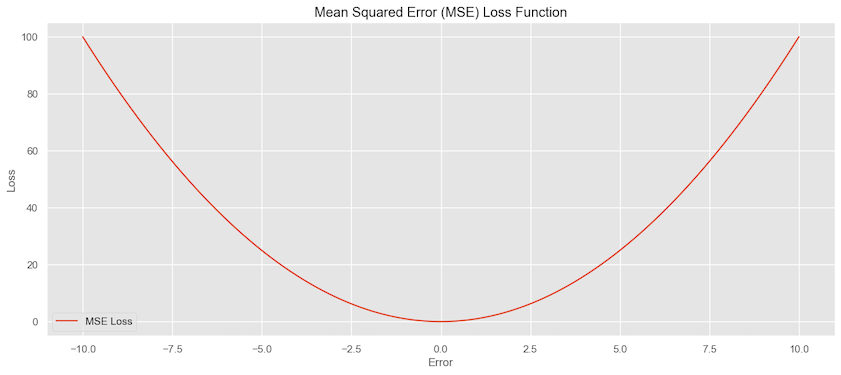
\[\hspace{5cm} \sum_{i=1}^{n}(y_{i}-(\beta_{0}+\beta_{1}x))^2\]This process finds the values of $\beta_{0}$ and $\beta_{1}$ that makes the sum as small as possible. The Mean squared loss function is convex and differentiable at each point as shown below.
Quantile Regression
In quantile regression, instead of finding the line that predicts the average $y$ for a given $x$, we find the lines that predict specific quantiles of $y$ for a given $x$. For instance, the median (50th percentile) or the 90th percentile. The quantile regression model for the $\tau^{th}$ quantile is:
\[\hspace{5cm} y = \beta_{0}(\tau)+\beta_{1}(\tau)x+\epsilon\]Here, $\tau$ represents the quantile of interest (e.g. $\tau =0.5$ for the median, $\tau=0.9$ for the 90th percentile).
To find the best fitting line for a specific quantile, we use a different approach than least squares. We minimize the sum of weighted absolute difference between the observed $y$ values and predicted $y$ values.For the $\tau^{th}$ quantile, the loss function is:
\[\hspace{5cm} \rho_{\tau}(u)=u(\tau-I(u<0))\]where:
- $u$ is the residual $(y_{i}-(\beta_{0}(\tau)+\beta_{i}(\tau)x_{i}))$.
- $\tau$ is the quantile (e.g. 0.5 for the median).
- $I(u \lt 0)$ is an indicator function that is 1 if $u$ is negative and 0 otherwise.
This loss function gives different weights to positive and negative residuals based on the quantile $\tau$. For instance, for median $\tau=0.5$, the loss function becomes:
\[\hspace{3cm} \rho_{0.5}(u)= \left\{ \begin{array}{cl} 0.5u & : u \geq 0 \\ 0.5u - u = -0.5u&: u < 0 \end{array} \right.\]This essentially treats positive and negative results equally, but for quantiles other than median, the weights differ.
Here is the plot for the quantile loss function for $0.1, 0.5 \text{ and } 0.9$ quantiles. we can see for the median quantile, the loss function is giving equal weight if the loss is positive or negative.
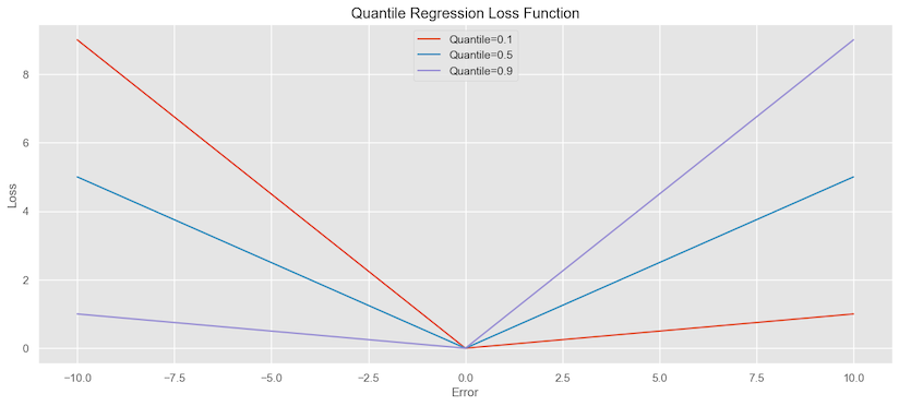
For the 0.1 quantile, the loss for negative errors (underestimation) has more weight, compared to the positive errors (overestimation). For 0.9 quantile, it’s the opposite, i.e. the weight for
negative errors is less and more on positive errors. The reason behind this is because for lower quantiles such as 0.1, the
regression aims to estimate a value such that 10% of the observations are below it. In this case, underestimation (negative errors)
is more concerning because we want to ensure that the estimated value is low enough to cover the bottom 10% of the data. For
higher quantile like 0.9, overestimation is more concerning because we want to ensure that estimated value is high enough to cover 90% of the data.
If we compare the loss function for Mean squared error in the linear regression which is smooth vs. Quantile loss function, it’s easy to see that quantile loss function is not differentiable at every point. The goal is to minimize the sum of the weighted absolute residuals and is solved using optimization techniques like linear programming.
\[\hspace{5cm} \sum_{i=1}^{n}\rho_{\tau}(y_{i}-(\beta_{0}(\tau)+\beta_{1}(\tau)x_{i}))\]Revisiting the Housing Sales Price Example
Let’s apply quantile regression and calculate 5th quantile (lower price range) and 95th percentile (higher end price range) indicated by the red and blue lines.
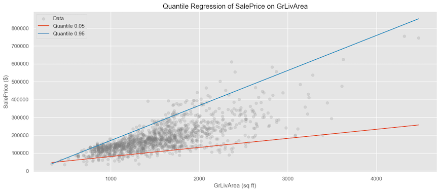
If we calculate the estimated price for 2500 sq. ft from the derived coefficients for the 5th and 95th percentiles, we get ~156K on the lower end and ~464K on the higher end. This is much better than having an average estimate of 300K.
If we want, we can look at the whole distribution by generating various quantiles.
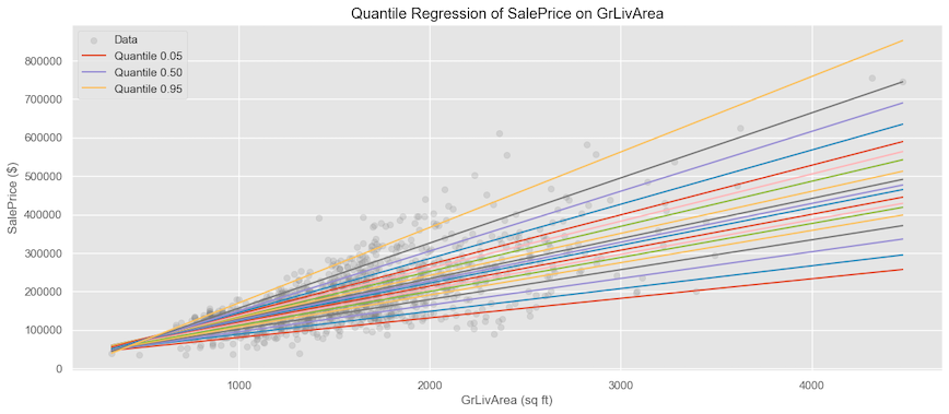
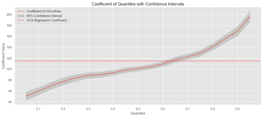
if we look at the change in the quantile coefficients and also plot the coefficients for the linear regression, we can see how as the quantiles increase, the coefficients increase vs. the flat linear regression coefficient.
LightGBM with Quantile Regression
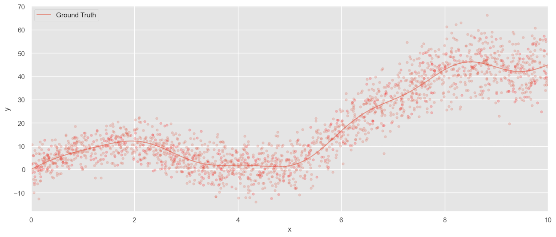
Here is another application example of Quantile regression on tree-based techniques. We have some synthetic data that becomes more variable as the value increases.
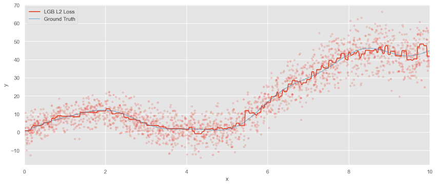
Using squared error loss, we have the predicted value versus the ground truth.
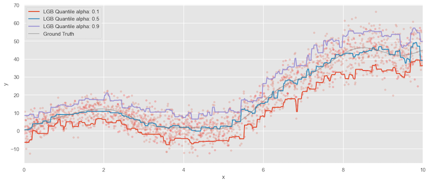
Now assuming Quantile regression and calculating for the 10th and 90th quantiles, we can see quantile regression captures the variability pretty well as the value of x increases.
Conclusion
In summary, quantile regression is an incredibly powerful and adaptable statistical method. Unlike traditional linear regression, which only focuses on modeling the mean, quantile regression allows us to model the entire conditional distribution of our response variable. This means we can gain insights into how different parts of the distribution, like the median, upper and lower quartiles, or even extreme quantiles, are affected by our predictors.
Quantile regression doesn’t require any assumptions about the distribution of the data. It lets us make predictions for specific quantile levels, while still controlling for other covariates.