Linear Regression Rough Notes
Introduction
When it comes to stats, one of the first topics we learn is linear regression. But many people don’t realize how deep the linear regression topic is. Below are my partial notes on Linear Regression for anyone who may find this helpful.

Linear Model
A basic statistical model with single explanatory variable has equation describing the relation between x and the mean
$\mu$ of the conditional distribution of Y at each value of x.
$ E(Y_{i}) = \beta_{0} + \beta_{1}x_{i} $
Alternative formulation for the model expresses $Y_{i}$
$ Y_{i} = \beta_{0} + \beta_{1}x_{i} + \epsilon_{i} $
where $\epsilon_{i}$ is the deviation of $Y_{i}$ from $E(Y_{i}) = \beta_{0} + \beta_{1}x_{i} + \epsilon_{i}$ is called
the error term, since it represents the error that results from using the conditional expectation of Y at $x_{i}$ to
predict the individual observation.
Least Squares Method
For the linear model $E(Y_{i}) = \beta_{0} + \beta_{1}x_{i}$, with a sample of n observations the least squares method determines the value of $\hat{\beta_{0}}$ and $\hat{\beta_{1}}$ that minimize the sum of squared residuals.
$ \sum_{i=1}^{n}(y_{i}-\hat{\mu_{i}})^2 = \sum_{i=1}^{n}[y_{i}-(\hat{\beta_{0}} + \hat{\beta_{1}}x_{i})]^2 = \sum_{i=1}^{n}e^{2}_{i} $
As a function of model parameters $(\beta_{0} , \beta_{1})$, the expression is quadratic in $\beta_{0},\beta_{1}$
$ S(\beta_{0} , \beta_{1}) = \sum_{i=1}^{n}(y_{i}-\hat{\mu_{i}})^2 = \sum_{i=1}^{n}[y_{i}-(\beta_{0} + \beta_{1}x_{i})]^2 $
We can minimize it w.r.t to $\beta_{0},\beta_{1}$ by
$ \frac{\partial S}{\partial \beta_{0}} = -\sum_{i=1}[y_{i}-(\beta_{0}+\beta_{1}x_{i})]=0 $
and
$ \frac{\partial S}{\partial \beta_{1}} = -\sum_{i=1}x_{i}[y_{i}-(\beta_{0}+\beta_{1}x_{i})]=0 $
We can rewrite the aboe equations as
$ \sum_{i=1}^{n}y_{i}= n\beta_{0}+\beta_{1}\sum_{i=1}^{n}x_{i} $
and
$ \sum_{i=1}^{n}x_{i}y_{i}= \beta_{0}(\sum_{i=1}^{n}x_{i})+\beta_{1}\sum_{i=1}^{n}x_{i}^2 $
Solution to the above equation yields
$ \hat{\beta_{0}} = \bar{y} - \hat{\beta_{1}}\bar{x}, \hat{\beta_{1}} = \frac{\sum_{i=1}^{n}(x_{i}-\bar{x})(y_{i}-\bar{y})}{\sum_{i=1}^{n}(x_{i} - \bar{x})^2} = \frac{s_{xy}}{s^2_{x}} $
where
$ s_{x}= \sqrt{\frac{\sum_{i}(x_{i}-\bar{x})^2}{(n-1)}} and s_{xy}= \frac{\sum_{i}(x_{i}-\bar{x})(y_{i} - \bar{y})}{(n-1)} $
$s_{x}$ is the sample standard deviation of x values and $s_{xy}$ is the sample covariance between x and y.
Example
Below is the Scottish Hill Runners Race data with distance and climb being explanatory
variable and record times being the response variable for Men and Women.
import random
import numpy as np
import pandas as pd
import matplotlib.pyplot as plt
import seaborn as sns
import scipy.stats as stats
from scipy.stats import t
from scipy.stats import norm
import statsmodels.stats.api as sms
import statsmodels.formula.api as smf
import statsmodels.api as sm
from statsmodels.stats.proportion import proportion_confint
from statsmodels.stats.outliers_influence import variance_inflation_factor

Races = pd.read_csv('data/ScotsRaces.dat', sep='\s+')
Races.head()

	race	distance	climb	timeM	timeW
0	AnTeallach	10.6	1.062	74.68	89.72
1	ArrocharAlps	25.0	2.400	187.32	222.03
2	BaddinsgillRound	16.4	0.650	87.18	102.48
3	BeinnLee	10.2	0.260	41.58	52.52
4	BeinnRatha	12.0	0.240	47.75	58.78

## Filtering Men times and plotting distance, climb and women times.
Races2 = Races.drop(['timeM'], axis=1)
sns.pairplot(Races2)
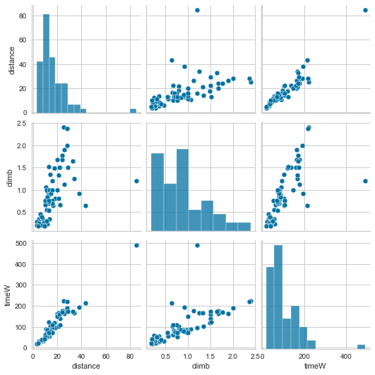
We can see correlation between timeW and distance, and timeW and climb. We also see some outlier.
Performing OLS between timeW and distance.
fitd = smf.ols(formula='timeW ~ distance', data=Races2).fit()
print(fitd.summary())
                            OLS Regression Results
==============================================================================
Dep. Variable:                  timeW   R-squared:                       0.913
Model:                            OLS   Adj. R-squared:                  0.912
Method:                 Least Squares   F-statistic:                     693.3
Date:                Sat, 15 Oct 2022   Prob (F-statistic):           1.00e-36
Time:                        16:30:34   Log-Likelihood:                -304.30
No. Observations:                  68   AIC:                             612.6
Df Residuals:                      66   BIC:                             617.0
Df Model:                           1
Covariance Type:            nonrobust
==============================================================================
                 coef    std err          t      P>|t|      [0.025      0.975]
------------------------------------------------------------------------------
Intercept      3.1076      4.537      0.685      0.496      -5.950      12.165
distance       5.8684      0.223     26.330      0.000       5.423       6.313
==============================================================================
Omnibus:                       12.420   Durbin-Watson:                   1.849
Prob(Omnibus):                  0.002   Jarque-Bera (JB):               13.203
Skew:                           0.913   Prob(JB):                      0.00136
Kurtosis:                       4.150   Cond. No.                         35.4
==============================================================================

print(fitd.params)
Intercept    3.107563
distance     5.868443
dtype: float64
The model fit $\hat\mu$ = 3.11 + 5.87(distance) indicates the predicted women’s record time increase by 5.87 minutes for every additional km of distance.
Multiple Linear Regression
The linear model with p explanatory variables, called multiple regression model is
$ E(Y_{i}) = \beta_{0} + \beta_{1}x_{i1} + …. + \beta_{p}x_{ip} $
where $E(Y_{i})$ represents the conditional expectation of the response variable at the values $(x_{i1},…,x_{ip})$ of the explanatory variables. To find the least squares estimates of the parameters, we minimize w.r.t parameters.
$ S(\beta_{0} , \beta_{1},…,\beta_{p}) = \sum_{i=1}^{n}(y_{i}-\hat{\mu_{i}})^2 = \sum_{i=1}^{n}[y_{i}-(\beta_{0} + \beta_{1}x_{i1}+…+\beta_{p}x_{ip})]^2 $
$ \frac{\partial S}{\partial \beta_{0}} = -\sum_{i=1}[y_{i}-(\beta_{0}+\beta_{1}x_{i1}+…+\beta_{p}x_{ip})]=0 $
$ \frac{\partial S}{\partial \beta_{j}} = -\sum_{i=1}x_{ij}[y_{i}-(\beta_{0}+\beta_{1}x_{i1}+…+\beta_{p}x_{ip})]=0, j = 1,…,p $
Example
expanding on the previous example by performing OLS between timeW vs distance and climb.
fitdc = smf.ols(formula="timeW ~ distance + climb", data=Races).fit()
print(fitdc.summary())
                            OLS Regression Results
==============================================================================
Dep. Variable:                  timeW   R-squared:                       0.964
Model:                            OLS   Adj. R-squared:                  0.963
Method:                 Least Squares   F-statistic:                     872.6
Date:                Sat, 15 Oct 2022   Prob (F-statistic):           1.10e-47
Time:                        17:02:00   Log-Likelihood:                -274.24
No. Observations:                  68   AIC:                             554.5
Df Residuals:                      65   BIC:                             561.1
Df Model:                           2
Covariance Type:            nonrobust
==============================================================================
                 coef    std err          t      P>|t|      [0.025      0.975]
------------------------------------------------------------------------------
Intercept    -14.5997      3.468     -4.210      0.000     -21.526      -7.674
distance       5.0362      0.168     29.919      0.000       4.700       5.372
climb         35.5610      3.700      9.610      0.000      28.171      42.951
==============================================================================
Omnibus:                        1.739   Durbin-Watson:                   1.805
Prob(Omnibus):                  0.419   Jarque-Bera (JB):                1.043
Skew:                          -0.158   Prob(JB):                        0.594
Kurtosis:                       3.518   Cond. No.                         53.5
==============================================================================

Notes:
[1] Standard Errors assume that the covariance matrix of the errors is correctly specified.
The model fit $\hat\mu$ = -14.6 + 5.04(distance) + 35.56(climb) indicates that adjusted for climb the predicted record time increases by 5.04mins for every additional km of distance. adjusted for distance, the predicted record time increases by 35.56mins for every additional km of climb.
The estimated conditional distance effect of 5.04 differs from the estimated marginal effect of 5.87 with distance as the sole explanatory variable because distance and climb are +ve correlated. With the climb in elevation fixed, distance has less of an effect than when the model ignores climb so that it also tends to increase as distance increases.
Leverage
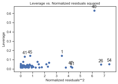
The leverage is a measure of an observation potential influence on the fit. Observations for which explanatory variables are far from their means have greater potential influence on the least square estimates.
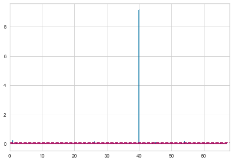
For an observation to actually be influential, it must have boths relatively large leverage and a relatively large residual. Cook’s distance uses both based on the change in $\beta_{j}$ when the observation is removed from the data set. For the residual $e_{i}$ and leverage $h_{i}$ for observation i, cook’s distance is
$ D_{i} = \frac{e_{i}^2h_{i}}{(p+1)s^2(1-h_{i})^2} $ where $s^2$ is an estimate of the conditional variance $\sigma^2$.
Cook’s distance is large when an observation has a large residual and a large leverage. The following code requests a plot of squared normalized residuals against the leverage:
sm.graphics.plot_leverage_resid2(fitdc)
influence = fitdc.get_influence()
leverage = influence.hat_matrix_diag
cooks_d = influence.cooks_distance
cooks_df = pd.DataFrame(cooks_d,index=['CooksDist','p-value'])
cooks_df = pd.DataFrame.transpose(cooks_df)
cooks_df.head(3)

	CooksDist	p-value
0	0.007997	0.999008
1	0.216293	0.884759
2	0.004241	0.999615
To identify values with high influence, we look for observations with:
- big blue points (high Cook’s distance) and
- high leverage (X-axis) which additionally have high or low studentized residuals (Y-axis).
fig = sm.graphics.influence_plot(fitdc, criterion="cooks")
fig.tight_layout(pad=1.0)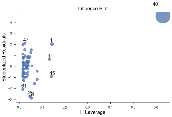
from yellowbrick.regressor import CooksDistance
X = Races.drop(['race', 'timeM', 'timeW'], axis=1)
y = Races['timeW']
visualizer = CooksDistance()
visualizer.fit(X, y)
X1 = X.loc[X.index != 40]
y1 = y.loc[y.index != 40]
visualizer = CooksDistance()
visualizer.fit(X1, y1)
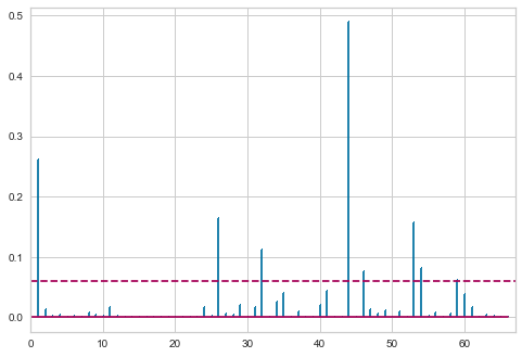
Repeating the OLS after removing the outlier.
Races2 = Races2.loc[~Races2.race.str.contains('Highland')]
fitdc2 = smf.ols(formula="timeW ~ distance + climb", data=Races2).fit()
print(fitdc2.summary())
                            OLS Regression Results
==============================================================================
Dep. Variable:                  timeW   R-squared:                       0.952
Model:                            OLS   Adj. R-squared:                  0.950
Method:                 Least Squares   F-statistic:                     634.3
Date:                Sat, 15 Oct 2022   Prob (F-statistic):           6.41e-43
Time:                        17:02:01   Log-Likelihood:                -261.27
No. Observations:                  67   AIC:                             528.5
Df Residuals:                      64   BIC:                             535.2
Df Model:                           2
Covariance Type:            nonrobust
==============================================================================
                 coef    std err          t      P>|t|      [0.025      0.975]
------------------------------------------------------------------------------
Intercept     -8.9315      3.281     -2.723      0.008     -15.485      -2.378
distance       4.1721      0.240     17.383      0.000       3.693       4.652
climb         43.8521      3.715     11.806      0.000      36.431      51.273
==============================================================================
Omnibus:                        1.552   Durbin-Watson:                   1.718
Prob(Omnibus):                  0.460   Jarque-Bera (JB):                0.871
Skew:                           0.174   Prob(JB):                        0.647
Kurtosis:                       3.437   Cond. No.                         46.9
==============================================================================

print ('R-Squared:', fitdc2.rsquared)
print ('Adjusted-Squared:', fitdc2.rsquared_adj)
fitted = fitdc2.predict()
print('Correlation between Time vs Fitted',np.corrcoef(Races2.timeW, fitted)[0,1])
residuals = fitdc2.resid
n=len(Races2.index); p=2
res_se = np.std(residuals)*np.sqrt(n/(n-(p+1)))
print ('residual standard error:', res_se)
print ('residual standard error**2:', res_se**2)
print ('Variance:',  np.var(Races2.timeW)*n/(n-1)) #estimated marginal variance

R-Squared: 0.9519750513925197
Adjusted-Squared:  0.9504742717485359
Correlation between Time vs Fitted 0.9756920884134089
residual standard error: 12.225327029914546
residual standard error**2: 149.4586209883592
Variance: 3017.7975421076458
Interaction between Explanatory Variables in their Effects
The equation $E(Y_{i}) = \beta_{0} + \beta_{1}x_{i1} + …. + \beta_{p}x_{ip}$ assumes that the relationship between $E(Y)$ and each $x_{j}$ is linear and that the slope $\beta_{j}$ of that relationship is identical at all values of the other explanatory variables.
The model containing only main effects is sometimes too simple. The effect of $x_{1}$ on y may change as the value
of $x_{2}$ changes, referred to as interaction between $x_{1}$ and $x_{2}$ in their effects.
A common approach for allowing interaction introduces cross-product terms of the explanatory variables in the model. With two explanatory variables, the model is
$ E(Y_{i}) = \beta_{0} + \beta_{1}x_{i1} + \beta_{2}x_{i2} + \beta_{3}x_{i1}x_{i2} $
To analyze how $E(Y_{i})$ relates to $x_{1}$, at different values for $x_{2}$, we rewrite the above equation in terms of $x_{1}$ as
$ E(Y_{i}) = (\beta_{0} + \beta_{2}x_{i2}) +(\beta_{1} + \beta_{3}x_{i2})x_{i1} = \beta_{0}^* + \beta_{1}^*x_{i1} $
where $\beta_{0}^* = \beta_{0} + \beta_{2}x_{i2}$ and $\beta_{1}^* = \beta_{1} + \beta_{3}x_{i2}$
For fixed $x_{2}$, $E(Y)$ changes linearly as a function of $x_{1}$. The slope of the relationship is $\beta_{1}^* = \beta_{1} + \beta_{3}x_{i2}$, so as $x_{2}$ changes, the slope for the effect of $x_{1}$ changes.
When the number of explanatory variables exceeds two, a model allowing interaction can contain cross-product terms for any pair of the explanatory variables. When a model includes an interaction term, it should have the hierarchical model structure by which it also contains the main effect terms that go into the interaction.
Example
For scottish hill race, it’s plausible that the effect of distance on record time is greater when the climb in elevation is greater. To allow the effect of distance to depend on the climb, we add an interaction term:
fitdc_int = smf.ols(formula='timeW ~ distance + climb + distance:climb',data=Races).fit()
print(fitdc_int.summary())
                            OLS Regression Results
==============================================================================
Dep. Variable:                  timeW   R-squared:                       0.966
Model:                            OLS   Adj. R-squared:                  0.964
Method:                 Least Squares   F-statistic:                     598.7
Date:                Sat, 15 Oct 2022   Prob (F-statistic):           9.45e-47
Time:                        16:48:59   Log-Likelihood:                -272.79
No. Observations:                  68   AIC:                             553.6
Df Residuals:                      64   BIC:                             562.5
Df Model:                           3
Covariance Type:            nonrobust
==================================================================================
                     coef    std err          t      P>|t|      [0.025      0.975]
----------------------------------------------------------------------------------
Intercept         -5.0162      6.683     -0.751      0.456     -18.367       8.335
distance           4.3682      0.433     10.083      0.000       3.503       5.234
climb             23.9446      7.858      3.047      0.003       8.247      39.643
distance:climb     0.6582      0.394      1.669      0.100      -0.129       1.446
==============================================================================
Omnibus:                        3.981   Durbin-Watson:                   1.813
Prob(Omnibus):                  0.137   Jarque-Bera (JB):                3.768
Skew:                          -0.244   Prob(JB):                        0.152
Kurtosis:                       4.045   Cond. No.                         196.
==============================================================================

Notes:
[1] Standard Errors assume that the covariance matrix of the errors is correctly specified.
It predicted negative time when distance=climb=0. We can make this fit a bit more realistic by constraining the
intercept term to equal 0. For a fixed climb value, the coefficient of distance in the prediction equation is
4.090 + 0.912(climb). Between the min climb of 0.185km and the max climb of 2.4km, the effect on record time of a 1km
increase in distance from 4.09+ 0.912(0.185) = 4.26 min to 4.09+0.912(2.4) = 6.28min.
# -1 constrains the intercept = 0
fitdc_int = smf.ols(formula='timeW ~ -1 + distance + climb + distance:climb',data=Races).fit()
print(fitdc_int.summary())

                                 OLS Regression Results
=======================================================================================
Dep. Variable:                  timeW   R-squared (uncentered):                   0.988
Model:                            OLS   Adj. R-squared (uncentered):              0.988
Method:                 Least Squares   F-statistic:                              1822.
Date:                Sat, 15 Oct 2022   Prob (F-statistic):                    1.22e-62
Time:                        16:49:16   Log-Likelihood:                         -273.09
No. Observations:                  68   AIC:                                      552.2
Df Residuals:                      65   BIC:                                      558.8
Df Model:                           3
Covariance Type:            nonrobust
==================================================================================
                     coef    std err          t      P>|t|      [0.025      0.975]
----------------------------------------------------------------------------------
distance           4.0898      0.223     18.338      0.000       3.644       4.535
climb             18.7128      3.616      5.176      0.000      11.492      25.934
distance:climb     0.9124      0.201      4.536      0.000       0.511       1.314
==============================================================================
Omnibus:                        3.866   Durbin-Watson:                   1.815
Prob(Omnibus):                  0.145   Jarque-Bera (JB):                3.983
Skew:                          -0.152   Prob(JB):                        0.136
Kurtosis:                       4.146   Cond. No.                         70.9
==============================================================================

Notes:
[1] R² is computed without centering (uncentered) since the model does not contain a constant.
[2] Standard Errors assume that the covariance matrix of the errors is correctly specified.
Residuals
Error terms being normally distributed
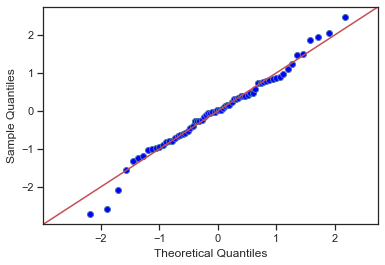
OLS requires error terms to follow normal distribution if we want to perform statistical hypothesis and generate reliable confidence and prediction intervals. To check for normality assumptions for residuals, use QQ and Histogram.
fitdc = smf.ols(formula="timeW ~ distance + climb", data=Races).fit()
fitted = fitdc.predict()
residuals = fitdc.resid

residuals.head()
0    13.170403
1    25.378848
2    11.371690
3     6.504777
4     4.410875
dtype: float64

plt.hist(residuals, density=False)
plt.xlabel('residuals'); plt.ylabel('frequencies')
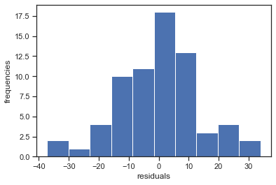
fig = sm.graphics.qqplot(residuals, dist=stats.norm, line='45', fit=True)
Jarque-Bera test The JB test is a goodness-of-fit test of whether sample data have the skewness and kurtosis matching a normal distribution.
The null hypothesis is a joint hypothesis of:
- the skewness being zero
- the kurtosis being 3
Samples from a normal distribution have an:
- an expected skewness of 0
- an expected excess kurtosis of 0 (which is the same as a kurtosis of 3).
Any deviation from this assumptions increases the JB statistic.
name = ['Jarque-Bera', 'Chi^2 two-tail prob.', 'Skew', 'Kurtosis']
test = sm.stats.jarque_bera(residuals)
lzip(name, test)

[('Jarque-Bera', 1.0429853552942074),
 ('Chi^2 two-tail prob.', 0.5936337824296948),
 ('Skew', -0.15821546700650482),
 ('Kurtosis', 3.5176716549501106)]
The p-value is above 0.05 and we can accept $H_{0}$. Therefore, the test gives us an indication that the errors are normally distributed.
Omnibus normtest Another test for normal distribution of residuals is the Omnibus normtest. The test allows us to check whether or not the model residuals follow an approximately normal distribution.
Our null hypothesis is that the residuals are from a normal distribution.
name = ['Chi^2', 'Two-tail probability']
test = sm.stats.omni_normtest(residuals)
lzip(name, test)
[('Chi^2', 1.738548720752564), ('Two-tail probability', 0.4192556674189445)]
The p-value is above 0.05 and we can accept $H_{0}$. Therefore, the test gives us an indication that the errors are from a normal distribution.
No AutoCorrelation among error terms
Another critical assumption of the linear regression model is that the error terms are uncorrelated. If they are not, then p-values associated with the model will be lower than they should be, and confidence intervals are unreliable.
Correlated errors mainly occur in the context of time series data. To determine if this is the case for a given data set, we can plot the residuals from our model as a function of time. If the errors are uncorrelated, then there should be no evident pattern. If the errors are uncorrelated, then the fact that $e_{i}$ is positive provides little or no information about the sign of $e_{i+1}$.
Correlation among the error terms can also occur outside of time series data. For instance, consider a study in which individuals’ heights are predicted from their weights. The assumption of uncorrelated errors could be violated if some of the individuals in the study are members of the same family, eat the same diet, or have been exposed to the same environmental factors.
Durbin-Watson test A test of autocorrelation that is designed to take account of the regression model is the Durbin-Watson test. It is used to test the hypothesis that there is no lag one autocorrelation in the residuals. This means if there is no lag one autocorrelation, then information about $e_{i}$ provides little or no information about $e_{i+1}$. A small p-value indicates there is significant autocorrelation remaining in the residuals. If there is no autocorrelation, the Durbin-Watson distribution is symmetric around 2.
As a rough rule of thumb:
- If Durbin–Watson is less than 1.0, there may be cause for concern.
- Small values of d indicate successive error terms are positively correlated.
- If d > 2, successive error terms are negatively correlated.
sm.stats.durbin_watson(residuals)
1.8045813026284943
Non-linearity
One crucial assumption of the linear regression model is the linear relationship between the response and the dependent variables. We can identify non-linear relationships in the regression model residuals if the residuals are not equally spread around the horizontal line (where the residuals are zero) but instead show a pattern, then this gives us an indication for a non-linear relationship. We can deal with non-linear relationships via basis expansions (e.g. polynomial regression) or regression splines.
Heteroscedasticity
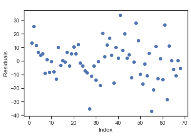
Another important assumption is that the error terms have a constant variance (homoscedasticity). For instance, the variances of the error terms may increase with the value of the response. One can identify non-constant variances in the errors, or heteroscedasticity by plotting the residuals and see if the variance appears to be uniform.
Heteroscedasticity can be solved either by using weighted least squares regression or transforming either the dependent or highly skewed variables. WLS assigns a weight to each data point based on the variance of its fitted value. Essentially, this gives small weights to data points that have higher variances, which shrinks their squared residuals. When the proper weights are used, this can eliminate the problem of heteroscedasticity.
Residual plots are a useful graphical tool for identifying non-linearity as well as heteroscedasticity. The residuals of this plot are those of the regression fit with all predictors.
index = list(range(1, len(residuals) + 1))
plt.scatter(index, residuals)
plt.title(' ')
plt.xlabel('Index'); plt.ylabel('Residuals')
plt.scatter(fitted, residuals)
plt.title(' ')
plt.xlabel('Fitted values'); plt.ylabel('Residuals')
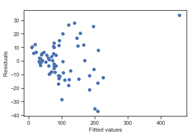
Breusch-Pagan Lagrange Multiplier test The Breusch-Pagan Lagrange Multiplier test can be used to identify heteroscedasticity. The test assumes homoscedasticity (this is the null hypothesis H0) which means that the residual variance does not depend on the values of the variables in x.
Note that this test may exaggerate the significance of results in small or moderately large samples. In this case the F-statistic is preferable.
If one of the test statistics is significant (i.e., p <= 0.05), then you have indication of heteroscedasticity.
name = ['Lagrange multiplier statistic', 'p-value', 'f-value', 'f p-value']
test = sm.stats.het_breuschpagan(fitdc.resid, fitdc.model.exog)
lzip(name, test)

[('Lagrange multiplier statistic', 26.85455722867833),
 ('p-value', 1.474371715752706e-06),
 ('f-value', 21.211902245960705),
 ('f p-value', 8.108058864393248e-08)]
P value is less than 0.05, means indication of hetroscedasity.
Partial Regression Plots
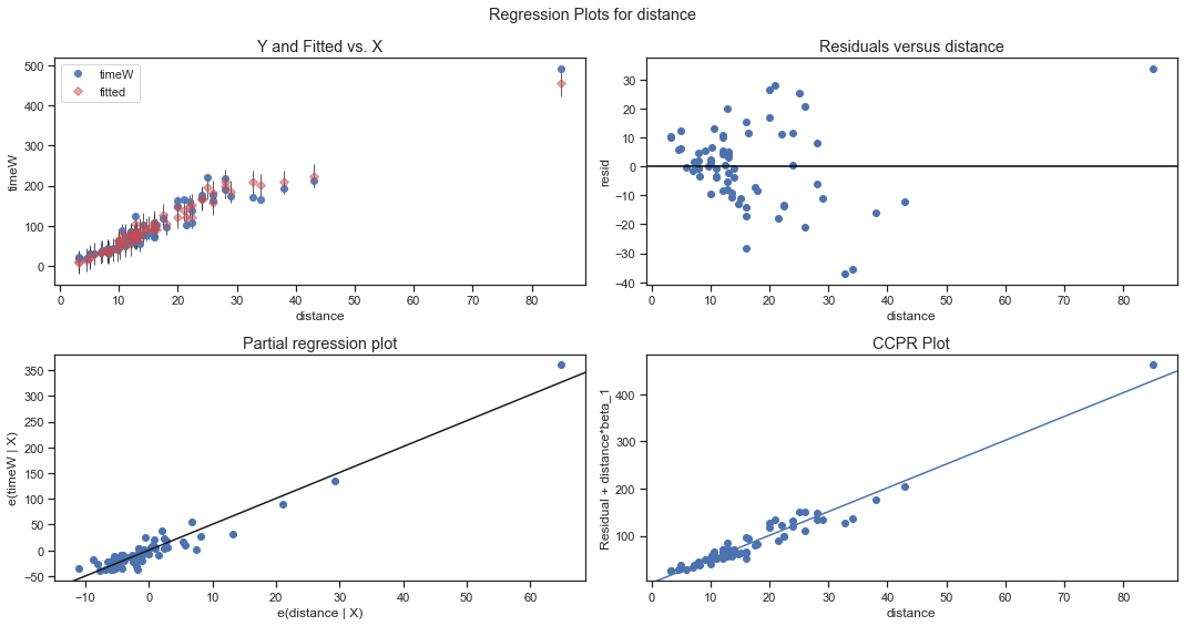
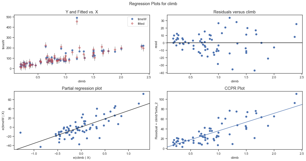
They are also called as Added-Variable Plots, where both the response variable $Y$ and the predictor variable under the investigation (like $X_{i}$) are both regressed against other predictor variables already in the regression model and the residuals are obtained for each. These two sets of residuals reflect the part of each ($Y$ and $X_{i}$) that is not linearly assosciated with the other predictor variables.
The plot of one set of residuals against the other set would show the marginal contribution of the candidate predictor in reducing variability as well as the information about the nature of its marginal distribution. For example, if we already have a regression model of $Y$ on predictor variable $X_{1}$ and is now considering if we should add $X_{2}$ into the model. In order to decide, we investigate
1) The regression of $Y$ on $X_{1}$ 2) The regression of $X_{2}$ on $X_{1}$
This gives us two sets of residuals. Then we do a regression of $e(Y|X_{1})$- as new dependent varibale on $e(X_{2}|X_{1})$- as independent variable. This gives us if the part of $X_{2}$ not contained in $X_{1}$ can further explained the part of $Y$ not explained in $X_{1}$.
CCPR PLOTS
The Component-Component plus Residual (CCPR) provides another way to judge the effect of one regressor on the response variable by considering the impact of the other independent variables. They are also a good way to see if the predictor has a linear relationship with the dependent variable. This plot, for a specific explanatory variable, say $X_{1}$=distance, plots the residuals plus the estimated linear effect of $X_{1}$ against $X_{1}$. It shows the relationship between $X_{1}$ and the response variable accounting for the remaining explanatory variables in the model.
The following code plots for each explanatory variable:
- Observed and fitted response values against the explanatory variable, including prediction intervals.
- residuals against the explanatory variable
- partial regression plots.
- CCPR plot.
sm.graphics.plot_regress_exog(fitdc, 'distance', fig=plt.figure(figsize=(15, 8)))
fig= sm.graphics.plot_regress_exog(fitdc,'climb',fig=plt.figure(figsize=(15, 8)))
Multicollinearity
Many times explanatory variables overlap considerably. Each variable may be nearly redundant because it can be predicted well using the others. So the effects in the multiple regression model may not be statistically significant even if highly significant marginally. Multicollinearity causes issues with the interpretation of the coefficients. You can interpret a coefficient as “an increase of 1 in this predictor results in a change of (coefficient) in the response variable, holding all other predictors constant.” This becomes problematic when multicollinearity is present because we can’t hold correlated predictors constant. Additionally, it increases the standard error of the coefficients, which results in them potentially showing as statistically insignificant when they might be significant.
Let $R_{j}^2$ denote $R^2$ from regressing $x_{j}$ on the other explanatory variables from the model. Then the estimated variance of $\hat\beta_{j}$ can be expressed as:
$ var(\hat\beta_{j}) = (se_{j})^2 = \frac{1}{(1-R_{j}^2)}\left[\frac{s^2}{(n-1)s^2_{xj}})\right] $
where $s^2_{xj}$ denotes the sample variance of $xj$ . The variance inflation factor
$ VIF_{j} = \frac{1}{(1-R^2_{j})} $
Multicollinearity can be fixed by other removing predictors with a high variance inflation factor (VIF) or performing dimensionality reduction.
VIF starts at one and has no upper limit. A value of 1 indicates there is no correlation. A value between 1 and 5 suggests a moderate correlation, but not severe enough. VIFs greater than 5 represent severe multicollinearity where the coefficients are poorly estimated.
X = Races2[['distance', 'climb']]
# VIF dataframe
vif_data = pd.DataFrame()
vif_data["feature"] = X.columns
# calculating VIF for each feature
vif_data["VIF"] = [variance_inflation_factor(X.values, i) for i in range(len(X.columns))]
print(vif_data)

    feature       VIF
0  distance  6.205809
1     climb  6.205809
R-squared
$TSS = SSR + SSE$ which in simple term means $Total Variablity = Explained Variability + Unexplained Variability$.
Mathematically we can express the above as:
$ \sum_{i}(y_{i} - \bar{y})^2= \sum_{i}(\hat\mu_{i} - \bar{y})^2 + \sum_{i}(y_{i} - \hat\mu_{i})^2 $
$R^2$ measures the proportional reduction in error which falls between 0 and 1.
$ R^2 = \frac{SSR}{TSS} = \frac{TSS-SSE}{TSS} = \frac{\sum_{i}(y_{i} - \bar{y})^2-\sum_{i}(y_{i} - \hat\mu_{i})^2}{\sum_{i}(y_{i} - \bar{y})^2} $
The least square fit minimizes SSE. When we add an explanatory variable to a model, SSE can not increase, because we could at worst obtain the same SSE value by setting $\hat\beta_{j}=0$ to a particular data set. SSR = TSS - SSE is montone increasing as the set of explanatory variable grows.
When n is not large and a model has several explantory variables, $R^2$ tends to overestimate the corresponding population value, which compares the marginal and conditional varinaces by the proportional reduction in variance.
An adjusted $R^2$ is designed to reduce this bias. It is proportional reduction in variance based on the unbiased variance estimates, $s^2_{y}$ for $var(Y)$ in the marginal distribution and $s^2$ for the variance in the conditional distributions; i.e.
$ Adjusted \space R^2 = 1 - \frac{n-1}{n-(p+1)}(1-R^2) $
It is slightly smaller than ordinary $R^2$, and it need not monotonically increase as explanatory variables are added to the model.
Inference for Normal Linear Models
Full Model
The “full model”, which is also sometimes referred to as the “unrestricted model,” is the model thought to be most appropriate for the data. For simple linear regression, the full model is:
$ Y_{i} = (\beta_{0} + \beta_{1}x_{i}) + \epsilon_{i} $
The question we have to answer is “does the full model describe the data well?”.
Residual Model
The “reduced model,” which is sometimes also referred to as the “restricted model,” is the model described by the null hypothesis. For simple linear regression, a common null hypothesis is. In this case, the reduced model is obtained by “zeroing out” the slope that appears in the full model. That is, the reduced model is:
$ Y_{i} = \beta_{0} + \epsilon_{i} $
This reduced model suggests that each response is a function only of some overall mean and some error.
F-Test
How do we decide if the reduced model or the full model does a better job of describing the trend in the data when it can’t be determined by simply looking at a plot? What we need to do is to quantify how much error remains after fitting each of the two models to our data. That is, we take the general linear test approach:
“Fit the full model” to the data.
- Obtain the least squares estimates of and .
- Determine the error sum of squares, which we denote as $SSE_{F}$.
“Fit the reduced model” to the data.
- Obtain the least squares estimate of .
- Determine the error sum of squares, which we denote as $SSE_{R}$.
$ F^* = \frac{SSE_{R}-SSE_{F}}{df_{R}-df_{F}}/(\frac{SSE_{F}}{df_{F}}) $
We use the general linear F-statistics to decide whether to
- Reject the null hypothesis: The reduced model
- In favor of the alternate hypothesis: The full model.
Conclusion
Don’t be Indiana Jones.