Introduction

I have always found TCP congestion control algorithms fascinating, and at the same time, I know very little about them. As an engineer working on the roads, it’s essential to understand the traffic requirement and service levels. Similarly, It’s good to understand the transport behavior riding our networks. Once in a while, I will feel guilty about it and spend time on the topic with the hope of gaining some new insights.

This blog post will share some of my experiments with various TCP congestion control algorithms. We will start with TCP Reno, then look at Cubic, and ends with BBR. I am using Linux network namespaces to emulate topology for experimentation, making it easier to run than setting up a physical test bed.

TCP Reno

For many years, the main algorithm of congestion control was TCP Reno. The goal of congestion control is to determine how much capacity is available in the network, so that source knows how many packets it can safely have in transit (Inflight). Once a source has these packets in transit, it uses the ACK’s arrival as a signal that packets are leaving the network, and therefore it’s safe to send more packets into the network. By using ACKs for pacing the transmission of packets, TCP is self-clocking. 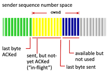The number of packets which TCP can inject into the network is controlled by Congestion Window(cwnd).

Congestion Window:

Reference: Computer Networking: A Top Down Approach

TCP states: Slow-Start, Congestion Avoidance and Fast-Recovery

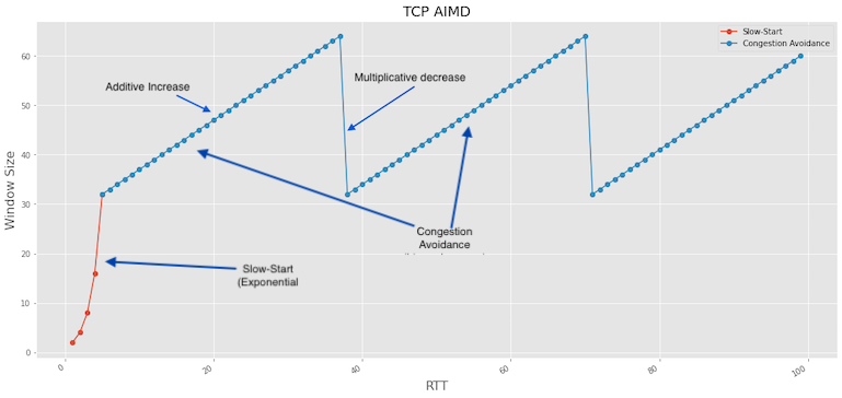
Slow-Start: TCP begins in Slow Start by sending certain number of segments, called the Initial window(IW). This can be somewhere between 2 and 4 segments based on the size of the MSS. For simplicity if we assume IW = 1 MSS and no packets are lost, an ACK is returned for the first segment, allowing sender to send another segment. If one segment is ACKed, the cwnd is increased to 2 and two segments are sent. We can represent this as $W = 2^k$ where k is the number of RTTs and W is the Window size in units of packets. As we can see, this is an exponential function highlighted in red in the graph below.

Congestion Avoidance: When the congestion window grows above a certain threshold known as ssthresh, it transitions to Congestion Avoidance phase, where the windows grow linearly. The window grows by $\frac{1}{cwnd}$ for each ACK received. This is the additive increase part of the AIMD strategy where the TCP tries to put packets in the network unless it detects a loss.

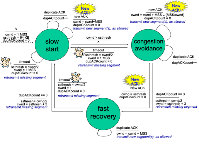
Fast-Recovery: If there is a packet loss, the TCP sender will receive a duplicate ACK (also called BAD ACks, which doesn’t return a higher ACK number). Rather than going back to Slow-Start, TCP enters the Fast-Recovery state, where it tries to recover from the Packet loss and moves back to the Congestion Avoidance phase once the recovery is complete. Reno Fast-Recovery was improved under New-Reno to handle multiple packet losses. During this state, TCP slows down by cutting cwnd by half, which is the Multiplicative decrease part of AIMD.

Here is the Finite State Machine for the TCP Reno:

Reference: Computer Networking: A Top Down Approach

TCP Reno Throughput

For modeling TCP Reno throughput, we have two well known equations

Mathis Equation for TCP Reno throughput:

\[\frac{MSS}{RTT}*\frac{1}{\sqrt{p}}\]

Padhye Equation for TCP Reno throughput:

\[min(\frac{W_{max}}{RTT}, \frac{1}{RTT\sqrt{\frac{2bp}{3}}+T_{0}min(1,3\sqrt{\frac{3bp}{8}})p(1+32p^{2})})\]

where p is the packet loss probability, $W_{max}$ is the max congestion window size and b is the number of packets of that are acknowledged by a received ACK.

Experiment

Single TCP Reno Session

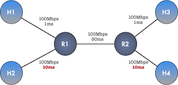
Now let’s get to the fun part. Let’s start with a simple topology of two hosts (H1, H2) connected by two routers(R1, R2). Router R1 has a small buffer of 100packets using FIFO queuing discipline. We will run a single TCP Reno session from host H1 to H2 for 200sec and observe the behavior on R1 and the host.

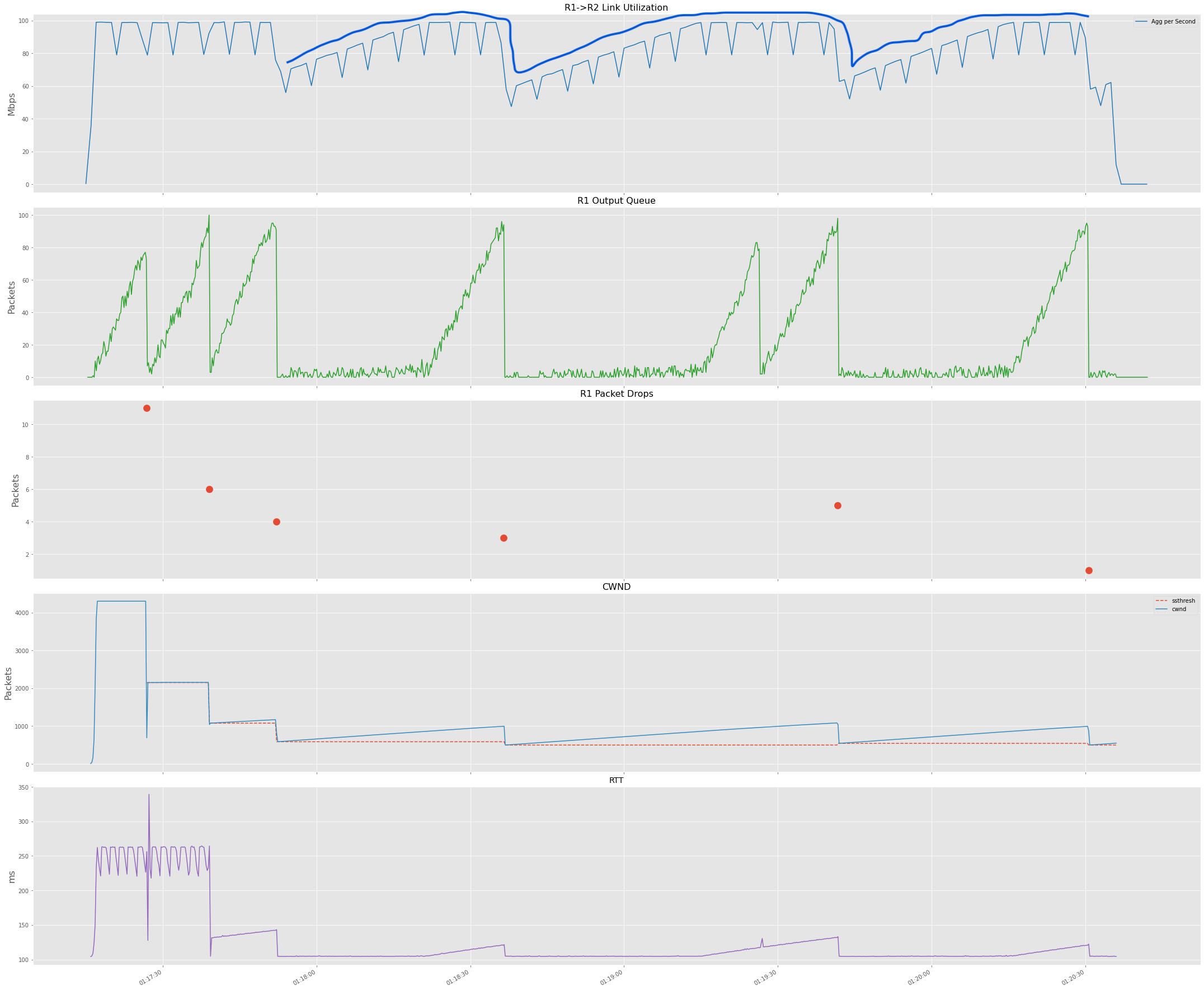
We collect stats at every 200ms from ss and tc, which should provide a good approximation. Link utilization is calculated by aggregating all the bytes transferred within a second and then converting them to Mbps. The below plot shows the results; the top three subplots show: R1 Link Utilization, R1 Output Queue, Packet Drops at R1, and the bottom two subplots show cwnd, ssthresh, and RTT observed.

The graph shows how TCP Reno fills queues, and you can see the corresponding bumps in RTT as the buffer fills up. As the sender experiences packet drops, the TCP receiver slows down by reducing its cwnd. You can also see the AIMD sawtooth pattern, which emerges in the link utilization.

Two TCP Reno Session

Now let’s add another host pair and have TCP session between H1->H3 and H2-H4 and repeat the experiment.

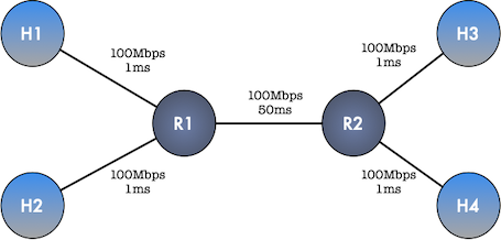
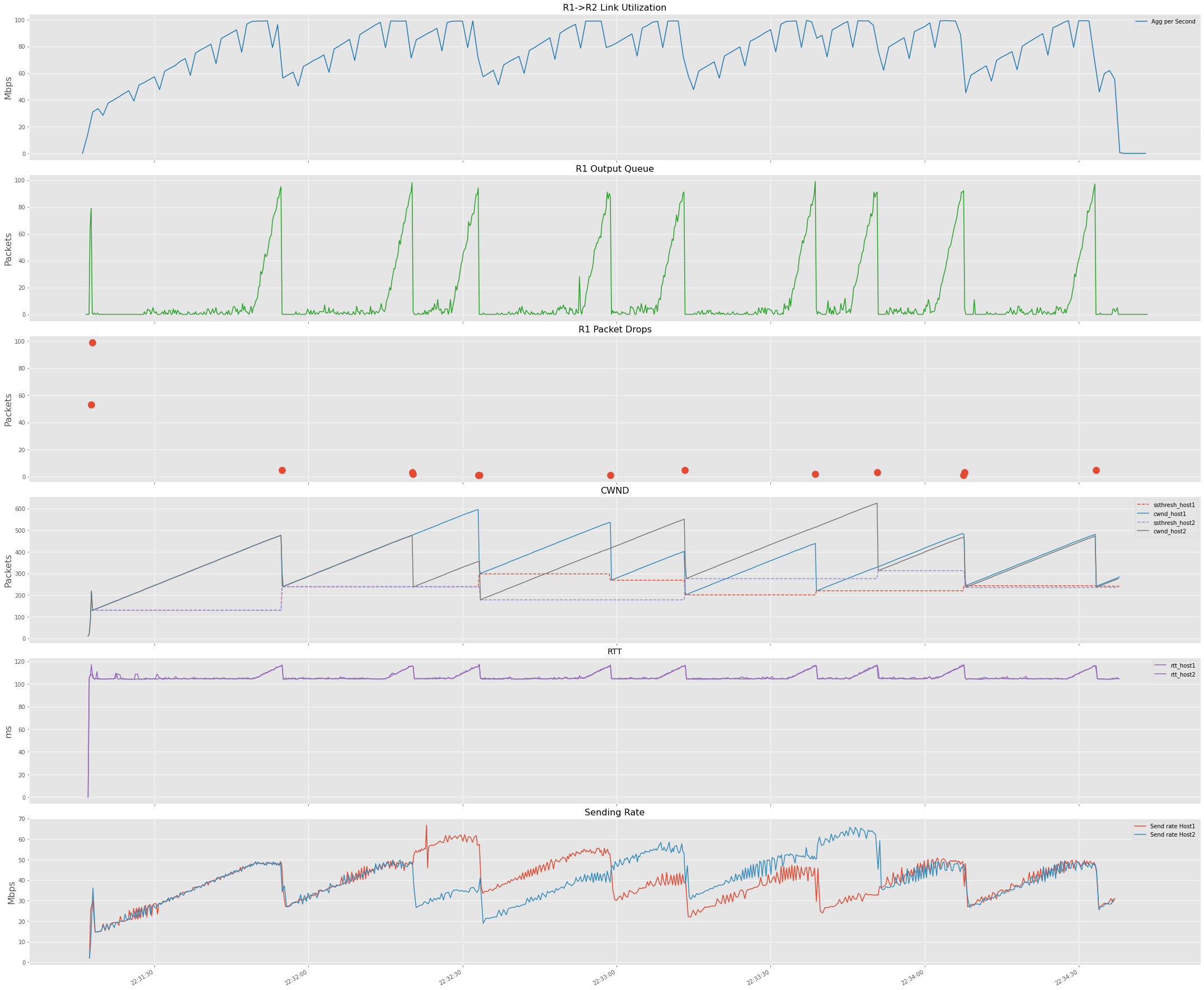
The below graph captures the results of the experiment. I have added the TCP sending rate for both hosts in this graph as well. In this case, both TCP sessions share the Router queue. We can see that buffer fills more frequently now, which should make sense due to the R1-R2 link being the bottleneck and both TCP senders collectively trying to push the maximum they can.

Also, looking at the TCP sending rate graph, we can see how both TCP sessions regulate each other.

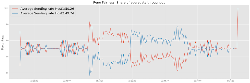
This brings the question of whether Reno TCP flows are fair to each other. Looking at the sum of sending rate for both hosts and percentage contribution of individual flows, We can see both TCP sessions fluctuate around ~50% and the average percentage for both flows is near 50%.

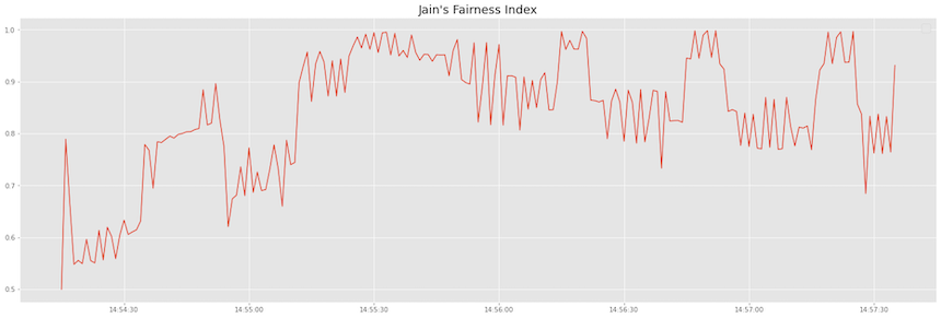
Formally we could also look at Jain’s index for measuring fairness which has the following properties:

1. Population size independence: the index is applicable to any number of flows.
2. Scale and metric independence: the index is independent of scale, i.e., the unit of measurement does not matter.
3. Boundedness: the index is bounded between 0 and 1. A totally fair system has an index of 1 and a totally unfair system has an index of 0.
4. Continuity: the index is continuous. Any change in allocation is reflected in the fairness index.

\[I = \frac{(\sum^{n}_{i=1}T_{i})^2}{n\sum^{n}_{i=1}T_{i}^2}\]

where

• I is the fairness index, with values between 0 and 1.
• n is the total number of flows.
• $T_{1}$, $𝑇_{2}$, . . . , $T_{n}$ are the measured throughput of individual flows.

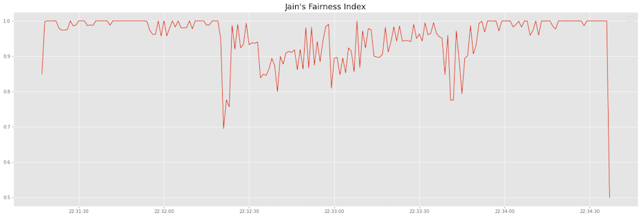
Plotting this for our two flows we see that how it fluctuates around 1 which is the perfect score.

RTT Unfairness

However, Because TCP Reno’s cwnd growth is proportional to RTT, a shorter RTT flow will be unfair to a longer RTT flow because of cwnd of the longer RTT flow will grow slowly. We can observe this by modifying the RTT for H2-H4. This will result in the flow H1-H3 taking more bandwidth share.

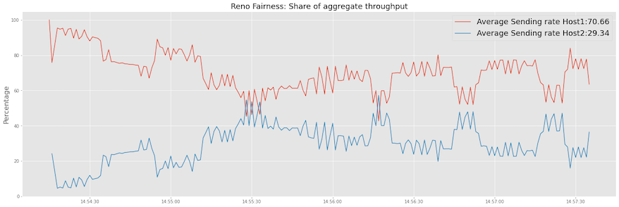
We can see that fairness index is not as close to 1 like it was in the previous case.

TCP Cubic

To provide higher throughput for large BDP networks, TCP Cubic (a modified version of BIC-TCP) came into the picture. This is currently the default congestion control algorithm for many operating systems. It’s still a loss-based congestion control algorithm that uses packet loss to indicate Congestion.

Reference: TCP CUBIC: A Transport Protocol for Improving the Performance of TCP in Long Distance High Bandwidth Cyber-Physical System

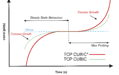
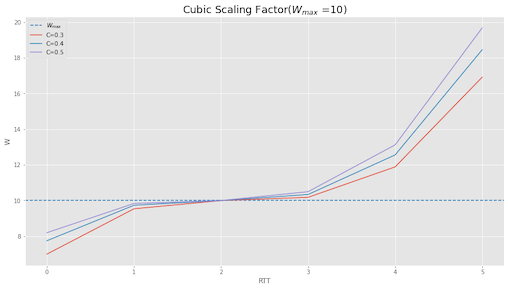
$W_{max}$ represents the window size where the loss occurs. Cubic decreases the cwnd by a constant decrease factor $\beta$ and enters into congestion avoidance phase and begins to increase cwnd size by using Eq. 1 as a concave feature of cubic function until the window size becomes $W_{max}$. The congestion window grows very fast after a window reduction, but as it gets close to $W_{max}$, it slows down its growth; around $W_{max}$, the window increment becomes almost zero.

\[W(t) = C(t-K)^3+W_{max} \qquad (Eq. 1)\] \[K = \sqrt[3]{\frac{W_{max}(1-\beta)}{C}}\]

where C is the scaling constant factor (default=0.4). C controls how fast the window will grow. $\beta$ is the multiplicative decrease factor after packet loss event, it’s default value is 0.7.t is the elapsed time from the last window reduction and K is the time period that the function requires to increase W to $W_{max}$.

The below plot shows the TCP Cubic function for scaling constant C with 0.3,0.4 and 0.5 values. We can see how for C=0.5, scales more aggressively than C=0.3.

Experiment

Two TCP Cubic sessions

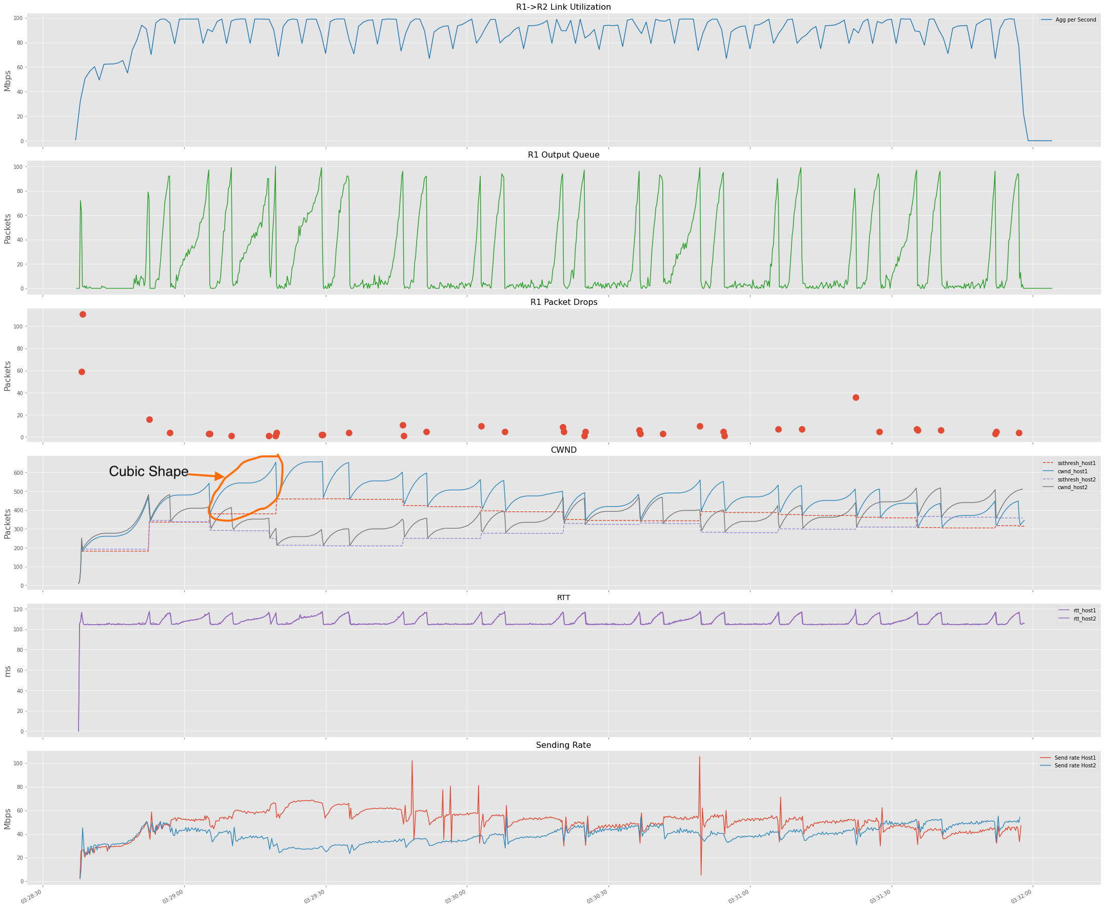
Repeating the experiment for two TCP Cubic sessions, below is the observed behavior. If you compare this with reno session output, you can see that the buffer fills are more frequent, which tells that window growth happens more aggressively. You can also observe the cubic function growth in the cwnd plot.

Cubic with Reno

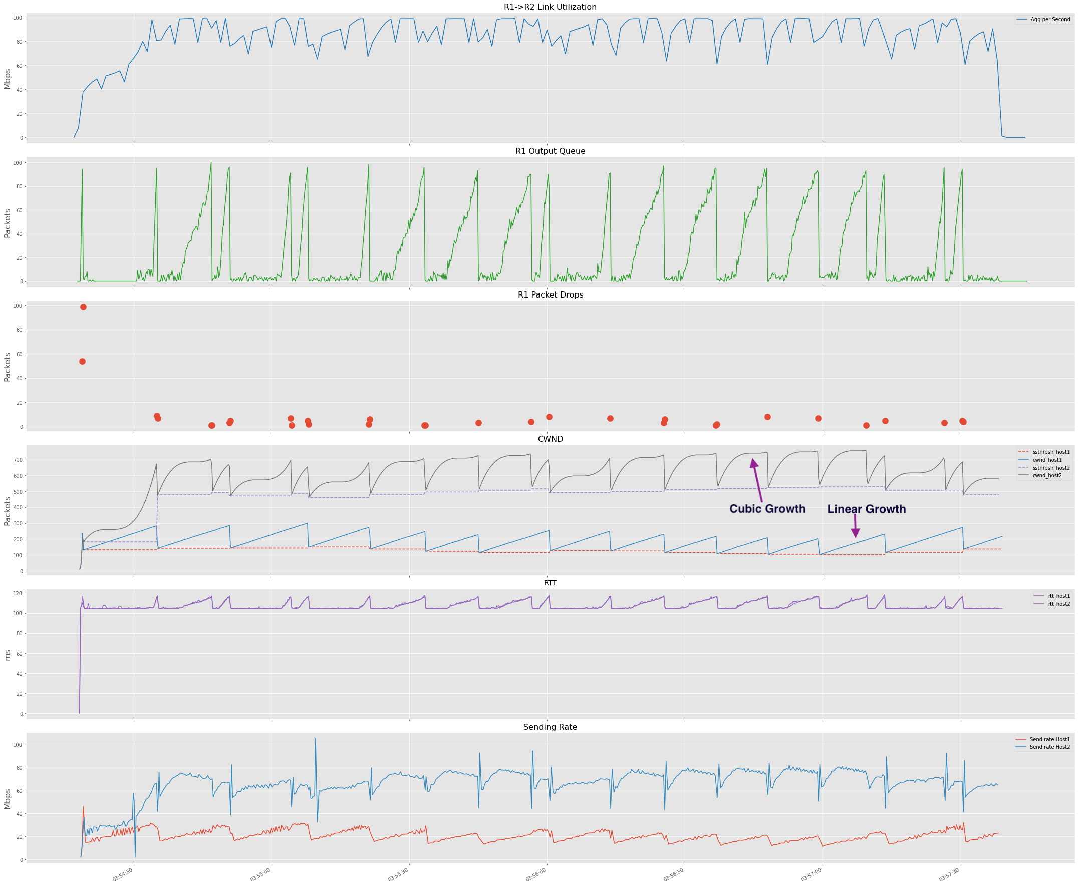
If we re-run the experiment with Host1 (H1-H3) running TCP Reno and Host2 (H2-H4) Cubic, we observe that TCP Cubic gets more bandwidth share. You can clearly see the differences in how the reno and cubic cwnd window growths.

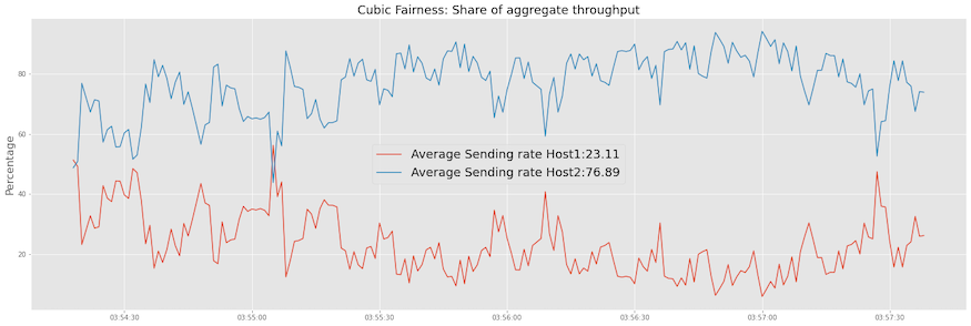
If we look at the bandwidth share, we clearly see Cubic taking the major share of the bandwidth.

TCP BBR

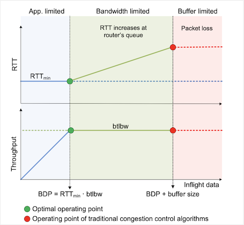
The BBR congestion control algorithm takes a different approach and does not assume that packet loss signals congestion. BBR builds a model of the network path to avoid and respond to actual congestion. In the case of BBR, at any given time, it sends data at a rate independent of current packet losses. This is a significant shift from traditional algorithms based on the AIMD rule, which operated by reducing the sending rate when they observed a packet loss.

BBR uses pacing to set the sending rate to the estimated bottleneck bandwidth. The pacing technique spaces out packets at the sender node, spreading them over time. This approach is a departure from the traditional loss-based algorithms, where the size of the congestion window establishes the sending rate, and the sender node may send packets in bursts up to the maximum rate of the sender’s interface.

The below figure describes the behavior of BBR, which show that BBR tries to operate at the optimal operating point, which is the Bandwidth delay product (BDP) highlighted in green, vs. the traditional algorithms, which operate at the BDP+Buffer size.

Reference: High-Speed Networks

To ensure that the sender adjusts to the increased bandwidth if there is an increase in available network bandwidth, BBR does periodic probing. It does by spending one RTT interval deliberately sending at a rate higher than the currently estimated bottleneck bandwidth. It sends data at 125% of the bottleneck bandwidth. If the available bottleneck bandwidth has not changed, the increased sending rate will cause a queue to form at the bottleneck link. This will cause the ACK signaling to reveal an increased RTT, and the sender will subsequently send at a compensating reduced sending rate for an RTT interval. The reduced rate is set to 75% of the bottleneck bandwidth, allowing the bottleneck queue to drain.

On the other hand, if the available bottleneck bandwidth estimate has increased because of this probe, then the sender will operate according to this new bottleneck bandwidth estimate.

Currently, TCP BBRv2 is in the beta stage, which addresses some BBRv1 shortcomings, like unfairness to other TCP Cubic flows.

Experiment

Two TCP BBR Session

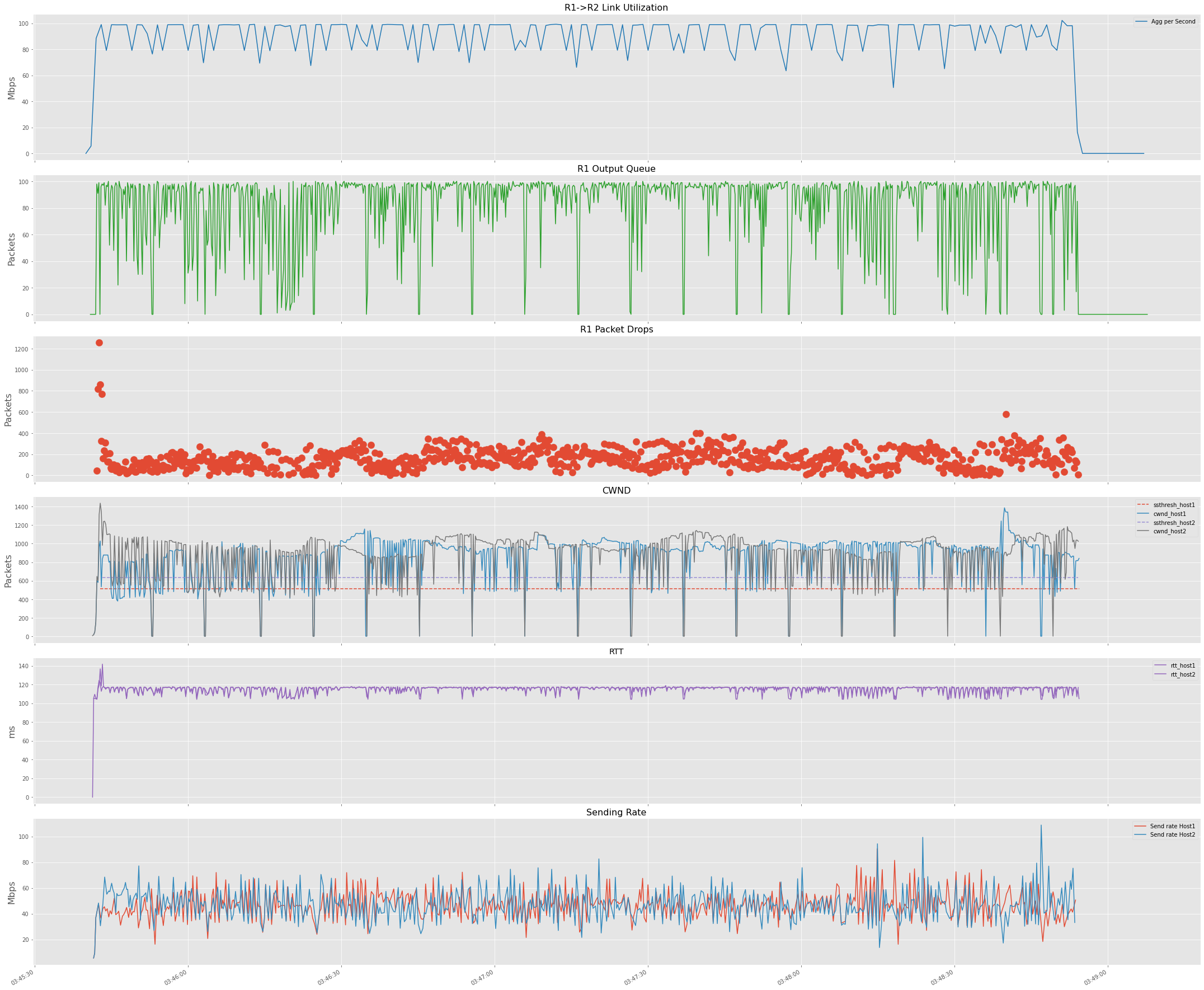
Let’s start by looking at two BBR sessions first. Some observations:

• Buffers are almost full. Please recall that our buffer here is 100 packets which are very shallow compared to the buffer required for BDP.
• Due to the shallow buffers and them always being full, we also observe more packet loss. However, the impact on throughput due to packet loss is not visible.
• Sender RTT estimates are pretty constant.
• Sending rate between both hosts seems to be approximately equal.

TCP BBR and Cubic Session

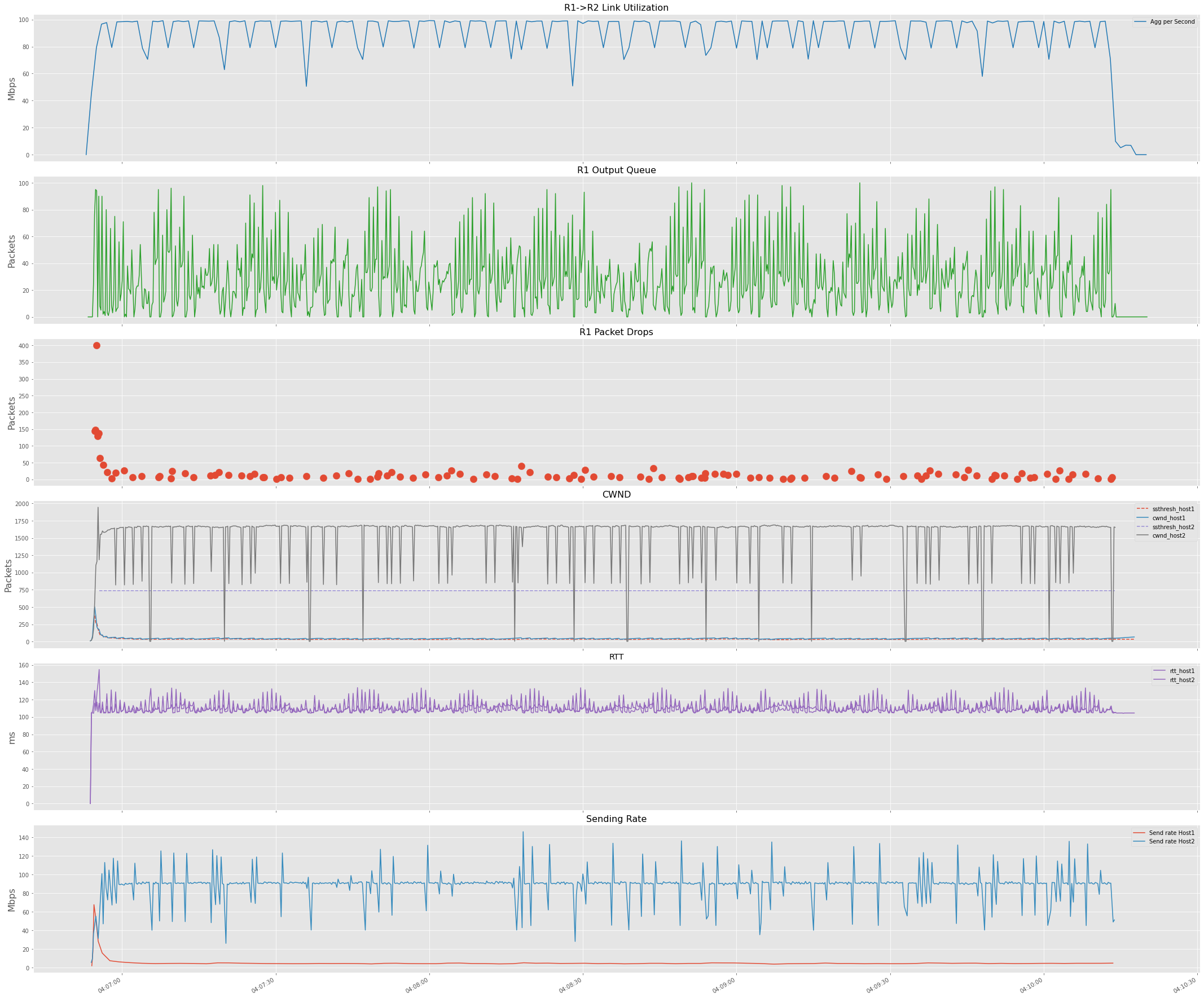
Now, if we change one session (H1-H3) from the previous experiment to TCP Cubic, we observe that BBR takes a fair share of the network bandwidth. This is due to buffers being less than BDP and TCP BBR not reacting to Loss while Cubic reacting to the packet loss and reducing its rate and thus ending up starved.

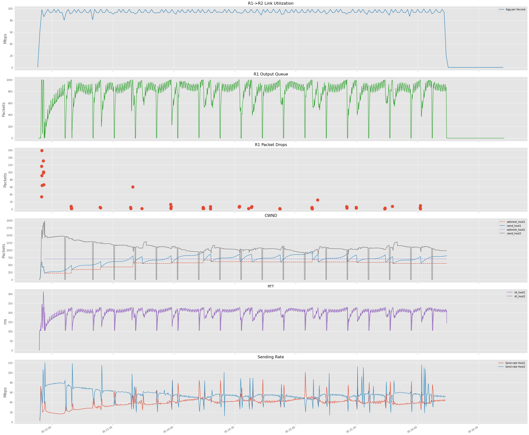
TCP BBR and Cubic Session with ~1xBDP

Let’s repeat the above experiment after increasing the buffer size on the router to 1000 Packets. Now we see a better resource sharing between BBR and Cubic.

Conclusion

In this blog post, we started with TCP Reno and looked at how Reno sessions are fair to each other and their bias towards RTT. Then we looked at TCP Cubic, differences in Reno vs. Cubic cwnd growth behavior, and how Cubic fairness compared to Reno. Then we finished with BBR and saw how the sending pace doesn’t slow with packet loss, and it’s unfairness towards Cubic with smaller buffers.

References

• TCP Cubic RFC8312
• TCP CUBIC: A Transport Protocol for Improving the Performance of TCP in Long Distance High Bandwidth Cyber-Physical System
• Towards a Deeper Understanding of TCP BBR Congestion Control
• BBR Congestion Control
• Modeling BBR’s Interactions With Loss-Based Congestion Control
• BBRv2
• Fairness Measure
• High-Speed Networks
• TCP/IP Illustrated
• TCP Congestion Control: A Systems Approach