Motivation

Clustering is a way to make sense of the data by grouping similar values into a group. There are many ways to achieve that and in this post we will be looking at one of the way based on spectral method. Spectral clustering provides a starting point to understand graphs with many nodes by clustering them into 2 or more clusters. This clustering technique can also be applied for analyzing general data. This technique is based on Linear algebra and Graph theory.

We will start with a very brief introduction of the prerequisite for the sake of completeness and one can skip the prerequisite topics if they already have the familiarity.

Prerequisite Topic

Eigen Vectors and Eigen Values

One way to interpret when we multiply a vector a matrix is that a matrix transforms the vector. For example: below is a vector \(\begin{pmatrix} 2\\1 \end{pmatrix}\)

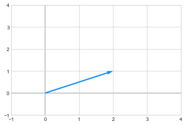
we apply a transformation by multiplying the above vector to a matrix

The resultant vector \(\begin{pmatrix} 1\\2 \end{pmatrix}\) is in orange after transformation.

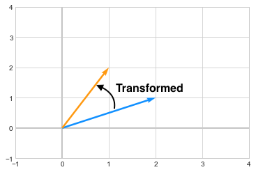
you can see how the vector changed its direction after the transformation. Now in case of Eigenvectors, which are special kinds of vectors on which, when we apply a transformation, they don’t change their direction. For example, assume we have a matrix A

The eigen vectors for this matrix are \(\begin{pmatrix} 1\\1 \end{pmatrix}\) and \(\begin{pmatrix} 1\\-3 \end{pmatrix}\). Multiplying the Matrix A to these vectors (hence applying a transformation to these vectors), only changes the length of these vectors by a certain value (i.e. eigen value) but it does not changes its direction. As you can see below, the vectors are scaled by 8 and 4 and those are the eigen values corresponding to those vectors.

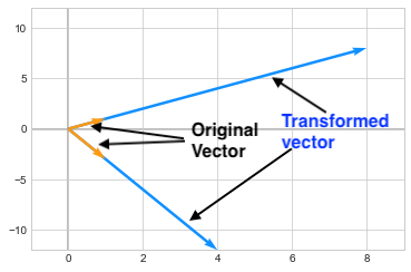
Mathematically we can express this by saying

$ Av = \lambda v $

So this concludes our one minute introduction of Eigen Vectors/Values with a hope that this brings some familiarity. There are lots of excellent resources out there where you can learn more about this.

Adjacency Matrix

A graph is a set of nodes with corresponding set of edges which connects the nodes. I am assuming most folks knows a bit about graphs. One way to represent a Graph is by Adjacency matrix. Below is a sample Graph

import numpy as np
import matplotlib.pyplot as plt
import networkx as nx
G3 = nx.Graph()
G3.add_nodes_from(np.arange(0,12))
edge_list = [(0,1), (0,4), (1,4),(1,2), (2,5), (2,3), (3,5),(4,5), (4,6), (5,7),(6,7),(6,8),(6,9),(8,9),
            (9,10), (7,10),(7,11), (10,11)]
G3.add_edges_from(edge_list)
fig, ax = plt.subplots(figsize=(9,7))
nx.draw_networkx(G3,pos=nx.spectral_layout(G3))

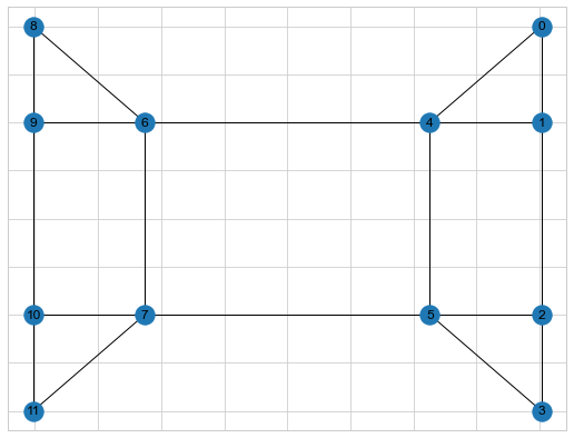
Adjancecy matrix for the above graph is shown below

A = np.array(nx.to_numpy_matrix(G3))
print(A)
##Output of A
[[0. 1. 0. 0. 1. 0. 0. 0. 0. 0. 0. 0.]
 [1. 0. 1. 0. 1. 0. 0. 0. 0. 0. 0. 0.]
 [0. 1. 0. 1. 0. 1. 0. 0. 0. 0. 0. 0.]
 [0. 0. 1. 0. 0. 1. 0. 0. 0. 0. 0. 0.]
 [1. 1. 0. 0. 0. 1. 1. 0. 0. 0. 0. 0.]
 [0. 0. 1. 1. 1. 0. 0. 1. 0. 0. 0. 0.]
 [0. 0. 0. 0. 1. 0. 0. 1. 1. 1. 0. 0.]
 [0. 0. 0. 0. 0. 1. 1. 0. 0. 0. 1. 1.]
 [0. 0. 0. 0. 0. 0. 1. 0. 0. 1. 0. 0.]
 [0. 0. 0. 0. 0. 0. 1. 0. 1. 0. 1. 0.]
 [0. 0. 0. 0. 0. 0. 0. 1. 0. 1. 0. 1.]
 [0. 0. 0. 0. 0. 0. 0. 1. 0. 0. 1. 0.]]

Degree Matrix

Degree matrix tells how many degrees each node has. For example, Node 8 has 2 degrees (connected to 9 and 6) and Node 6 has 4 degrees. We can compute the degrees from the adjacency matrix as well by counting the number of adjacency. Below is the degree matrix of the above graph

D = np.diag(A.sum(axis=1))
print(D)
## Degree Matrix
[[2. 0. 0. 0. 0. 0. 0. 0. 0. 0. 0. 0.]
 [0. 3. 0. 0. 0. 0. 0. 0. 0. 0. 0. 0.]
 [0. 0. 3. 0. 0. 0. 0. 0. 0. 0. 0. 0.]
 [0. 0. 0. 2. 0. 0. 0. 0. 0. 0. 0. 0.]
 [0. 0. 0. 0. 4. 0. 0. 0. 0. 0. 0. 0.]
 [0. 0. 0. 0. 0. 4. 0. 0. 0. 0. 0. 0.]
 [0. 0. 0. 0. 0. 0. 4. 0. 0. 0. 0. 0.]
 [0. 0. 0. 0. 0. 0. 0. 4. 0. 0. 0. 0.]
 [0. 0. 0. 0. 0. 0. 0. 0. 2. 0. 0. 0.]
 [0. 0. 0. 0. 0. 0. 0. 0. 0. 3. 0. 0.]
 [0. 0. 0. 0. 0. 0. 0. 0. 0. 0. 3. 0.]
 [0. 0. 0. 0. 0. 0. 0. 0. 0. 0. 0. 2.]]

Laplacian Matrix or Graph Laplacian

At this point, you already know what an Adjacency and Degree matrix are. Laplacian matrix or Graph Laplacian is given by

$ L = Degree Matrix - Adjacency Matrix $

In our example, we get the following Laplacian matrix for our graph

L = D - A
print(L)
## Output
[[ 2. -1.  0.  0. -1.  0.  0.  0.  0.  0.  0.  0.]
 [-1.  3. -1.  0. -1.  0.  0.  0.  0.  0.  0.  0.]
 [ 0. -1.  3. -1.  0. -1.  0.  0.  0.  0.  0.  0.]
 [ 0.  0. -1.  2.  0. -1.  0.  0.  0.  0.  0.  0.]
 [-1. -1.  0.  0.  4. -1. -1.  0.  0.  0.  0.  0.]
 [ 0.  0. -1. -1. -1.  4.  0. -1.  0.  0.  0.  0.]
 [ 0.  0.  0.  0. -1.  0.  4. -1. -1. -1.  0.  0.]
 [ 0.  0.  0.  0.  0. -1. -1.  4.  0.  0. -1. -1.]
 [ 0.  0.  0.  0.  0.  0. -1.  0.  2. -1.  0.  0.]
 [ 0.  0.  0.  0.  0.  0. -1.  0. -1.  3. -1.  0.]
 [ 0.  0.  0.  0.  0.  0.  0. -1.  0. -1.  3. -1.]
 [ 0.  0.  0.  0.  0.  0.  0. -1.  0.  0. -1.  2.]]

As you can see, the above matrix is a sparse symmetric matrix. Symmetric matrices have lot of nice properties and one of the main property is that all Eigen values are real. Any symmetric matrix can be decomposed by \(S = Q\Lambda Q^{t}\), where \(Q\) is the matrix containing orthogonal eigen vectors and \(\Lambda\) containing Eigen values which is what spectral theorem tells us. The world “Spectral” in Spectral Clustering indicates that this technique has something to do with the Eigen Values.

Eigenvalues of Graph Laplacian

Below are the Eigen Values for the graph Laplacian of our sample graph.

fig, (ax1,ax2) = plt.subplots(nrows=1, ncols=2, figsize=(15,5))
nx.draw_networkx(G3,pos=nx.spectral_layout(G3), ax=ax1)
G3_L = nx.laplacian_matrix(G3).toarray()
vals, vecs = np.linalg.eig(G3_L)
# sort these based on the eigenvalues
vecs = vecs[:,np.argsort(vals)]
vals = vals[np.argsort(vals)]
x = np.arange(1, G3_L.shape[0]+1)
ax2.scatter(x, vals)
ax2.set_xlabel("Eigen Vectors", fontsize=12)
ax2.set_ylabel("Eigen Values", fontsize=12)

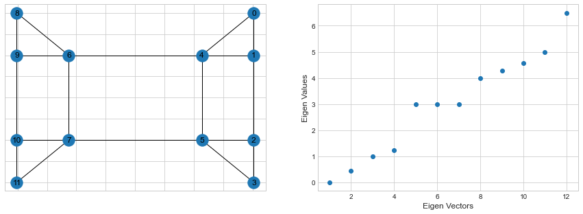
First Eigen value is zero for the first eigen vector and all other eigen values are positive. This also means that the matrix is positive semi-definite.

The second eigen vector which has a positive eigen value is known as Fiedler vector. Eigen value for the fiedler vector (second eigen value) tells us about the strength of the graph connectivity.

Fiedler eigen value is also known as Algebraic connectivity in Graph theory.

#second eigen value
vals[1]
0.43844718719116876

#algebraic connectivity
nx.algebraic_connectivity(G3)
0.43844718719117043

Below is the corresponding Fiedler vector

vecs[:,1]
### Fiedler Vector
array([ 0.32859615,  0.32859615,  0.32859615,  0.32859615,  0.18452409,
        0.18452409, -0.18452409, -0.18452409, -0.32859615, -0.32859615,
       -0.32859615, -0.32859615])

G3.nodes
## Node ordering
NodeView((0, 1, 2, 3, 4, 5, 6, 7, 8, 9, 10, 11))

You can see that few values are postive and remaining are negative. Fiedler vector shows that if we have to split the graph into two clusters, than the positive values belong to one cluster and negative values belong to second cluster. Which in our examples translates into 0,1,2,3,4,5 into one cluster and 6,7,8,9,10,11 into another cluster which makes sense.

In general, one looks at the first biggest gap between eigen values to get an idea on the number of clusters present in a graph. In our example, we can see that that first biggest gap is between 4 and 5, indicating that the graph contains around 4 clusters.Let’s use the Sci-kit learn this time to look at those 4 clusters:

from sklearn.cluster import SpectralClustering
#Converts graph to an adj matrix.
adj_matrix = nx.to_numpy_matrix(G3)
node_list = list(G3.nodes()) 

clusters = SpectralClustering(affinity = 'precomputed', assign_labels="discretize",random_state=0,n_clusters=4).fit_predict(adj_matrix)
plt.scatter(node_list,clusters,c=clusters, s=50, cmap='viridis')
plt.show()

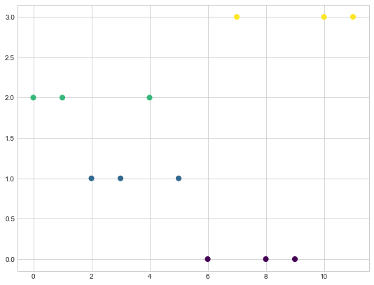
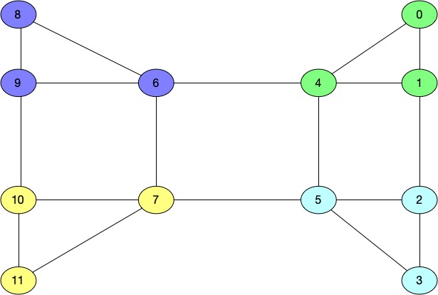
As you can see based on the colors for the nodes, we have following clusters in our graph.

Cluster1 - 6,8,9
Cluster2 - 2,3,5
Cluster3 - 0,1,4
Cluster4 - 7,10,11

Strength of a Graph or Algebraic Connectivity

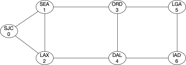
As I mentioned earlier that Fiedler value tells us about the strength of a graph. Let’s look at this by looking at an example. Assume that we have a graph like this (assume it’s a backbone network):

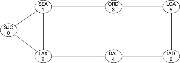
As you can see, the topology most looks like a ring and the algebraic connectivity score is around 0.75302.

G4= nx.Graph()
G4.add_nodes_from(np.arange(0,7))
edge_list = [(0,1), (0,2), (1,2), (1,3), (3,5), (5,6), (4,6), (2,4)]
G4.add_edges_from(edge_list)
G4_L = nx.laplacian_matrix(G4).toarray()
vals, vecs = np.linalg.eig(G4_L)
vecs = vecs[:,np.argsort(vals)]
vals = vals[np.argsort(vals)]
vals[1].round(5)
## Algebraic connectivity score
0.75302

Min-Cut for the graph is 2, i.e. the network will get partitioned with two cuts. Now let’s add a link between ORD-DAL and see what our score looks like.

G4.add_edge(3,4)
G4_L = nx.laplacian_matrix(G4).toarray()
vals, vecs = np.linalg.eig(G4_L)
# sort these based on the eigenvalues
vecs = vecs[:,np.argsort(vals)]
vals = vals[np.argsort(vals)]
vals[1].round(5)
## Algebraic connectivity score
0.75302

It doesnt seems it improved at all. That’s because from a topology strength prespective, we still have two min-cuts which will partition the topology into two complete graphs. Let’s add a link between ORD-IAD and then between SEA-DAL.

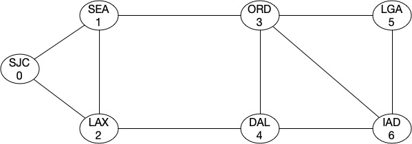
G4.add_edge(3,6)
G4_L = nx.laplacian_matrix(G4).toarray()
vals, vecs = np.linalg.eig(G4_L)
# sort these based on the eigenvalues
vecs = vecs[:,np.argsort(vals)]
vals = vals[np.argsort(vals)]
vals[1].round(5)
## Algebraic connectivity score
0.81435

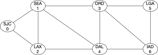
G4.add_edge(1,4)
G4_L = nx.laplacian_matrix(G4).toarray()
vals, vecs = np.linalg.eig(G4_L)
# sort these based on the eigenvalues
vecs = vecs[:,np.argsort(vals)]
vals = vals[np.argsort(vals)]
vals[1].round(5)
## Algebraic connectivity score
0.91387

You can see that our algebraic connectivity score aka the strength of topology increased in both cases as we introduced those links.

Spectral Clustering for General Data

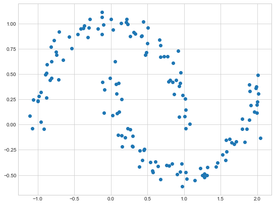
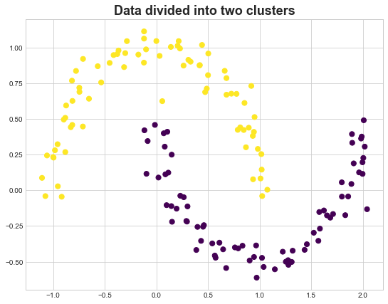
We can also apply this technique on general data. The trick is to convert the datapoints into a graph first. One way to do that is based on some notion of distance, for example, if two datapoints are very close to each other, there is an edge between them. Below is a sample example

from sklearn.cluster import SpectralClustering
from sklearn.datasets import make_moons
random_state = 21
dot_size=50
cmap = 'viridis'
X_mn, y_mn = make_moons(150, noise=.07, random_state=random_state)
fig, ax = plt.subplots(figsize=(9,7))
plt.scatter(X_mn[:, 0], X_mn[:, 1])

from sklearn.neighbors import radius_neighbors_graph
A = radius_neighbors_graph(X_mn,0.4,mode='distance', metric='minkowski', p=2, metric_params=None, include_self=False)
A = A.toarray()
D = np.diag(A.sum(axis=1))
L = D - A
vals, vecs = np.linalg.eig(L)
# sort these based on the eigenvalues
eigvecs = vecs[:,np.argsort(vals)]
eigvals = vals[np.argsort(vals)]
y_spec =eigvec[:,1].copy()
y_spec[y_spec < 0] = 0
y_spec[y_spec > 0] = 1
fig, ax = plt.subplots(figsize=(9,7))
ax.set_title('Data divided into two clusters', fontsize=18, fontweight='demi')
ax.scatter(X_mn[:, 0], X_mn[:, 1],c=y_spec ,s=dot_size, cmap=cmap)

References

Linear Algebra and Learning from Data
A Tutorial on Spectral Clustering