Maximum Flow Problems
Introduction
In optimization theory, Maximum Flow problems involve finding the maximum flow (or traffic) that can be sent from one place to another, subject to certain constraints. In this post, we will look at Maximum Flow algorithms applied to Networking and the questions they can help answer.
The main focus here will be the applied part, and we will only cover the surface of most algorithms as many of them requires Linear Programming and Optimization theory background.
Problem Setup
Assume that we have a small network connecting a few locations in the US using RSVP-TE for traffic management.
RSVP-TE allows us to find paths if there is not enough room on the shortest path, which removes the restriction that the
flows need to travel only on the shortest path.
In the below picture, we can see the Capacity and IGP cost of the links. From a graph representation perspective,
we will use MultiDigraph. Multi to represent multiple links, like between lax<-->iad, and Digraph for capturing the
unidirectional behavior of RSVP LSPs.
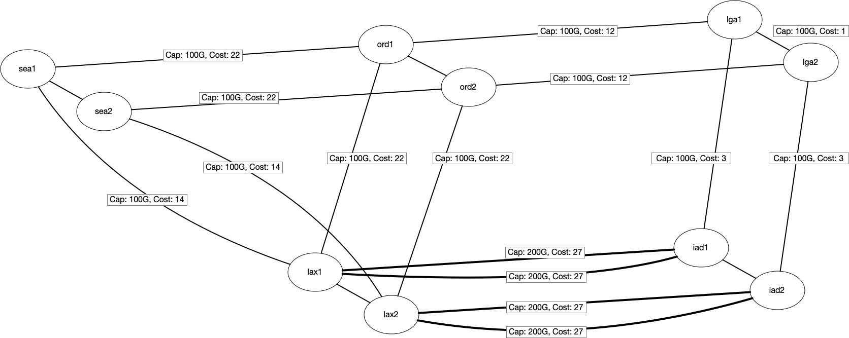
We will also assume that we already have some traffic routed between a few locations. The below table shows the existing traffic traveling between locations. For example, we have 100Gbps between LAX <-> IAD 100Gbps. Similarly, 100Gbps between SEA <-> IAD.
DEMANDS TABLE
lax,iad,100
iad,lax,100
sea,iad,100
iad,sea,100
Also, assume that 75% of the link capacity is available for RSVP, and the maximum size of a given RSVP LSP can not be
more than 5Gbps. This means that if the RSVP LSP needs to carry more than 5Gbps, it will be split into multiple LSPs.
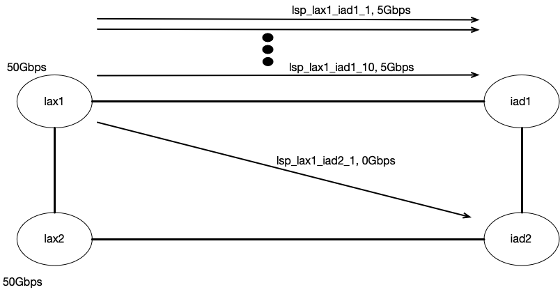
For instance, Let’s say the traffic between lax-iad needs to carry 50Gbps of traffic; we will have at least ten parallel
RSVP LSPs between them with a max size of LSPs around 5Gbps.
We will require some help from simulation tools to replicate the current network state, including the topology and routing the current demands between locations via LSPs.
model = Model.load_model("test_topology.csv")     # Load the topology file
model.interfaces.initialize_latency()             # Initialize the latency
model.simulate                                    # Route the Model
The simulation tool also makes sure it models the behavior of LSPs where only the LSPs with metric equal to the shortest
path IGP metric carries traffic. For example, LSPs between
lax1 - iad1 will carry the traffic in this simple square topology, and lax1 - iad2 will remain empty. Also, the
creation and deletion of parallel LSPs are dynamic.
After simulating the current state, if I look at the Interface utilization and Routing state, I see that RSVP LSPs between
SEA -> IAD are using the SEA -> ORD -> LGA -> IAD as there is enough bandwidth on the shortest path to satisfy the
current demands. The same thing applies to LAX -> IAD.
Demand: dmd_sea2_iad2, Traffic: 50.0Gbps
LSP Name: lsp_sea2_iad2_1, Traffic: 5.0Gbps, Path: ['sea2-to-ord2', 'ord2-to-lga2', 'lga2-to-iad2']
LSP Name: lsp_sea2_iad2_2, Traffic: 5.0Gbps, Path: ['sea2-to-ord2', 'ord2-to-lga2', 'lga2-to-iad2']
LSP Name: lsp_sea2_iad2_3, Traffic: 5.0Gbps, Path: ['sea2-to-ord2', 'ord2-to-lga2', 'lga2-to-iad2']
LSP Name: lsp_sea2_iad2_4, Traffic: 5.0Gbps, Path: ['sea2-to-ord2', 'ord2-to-lga2', 'lga2-to-iad2']
LSP Name: lsp_sea2_iad2_5, Traffic: 5.0Gbps, Path: ['sea2-to-ord2', 'ord2-to-lga2', 'lga2-to-iad2']
LSP Name: lsp_sea2_iad2_6, Traffic: 5.0Gbps, Path: ['sea2-to-ord2', 'ord2-to-lga2', 'lga2-to-iad2']
LSP Name: lsp_sea2_iad2_7, Traffic: 5.0Gbps, Path: ['sea2-to-ord2', 'ord2-to-lga2', 'lga2-to-iad2']
LSP Name: lsp_sea2_iad2_8, Traffic: 5.0Gbps, Path: ['sea2-to-ord2', 'ord2-to-lga2', 'lga2-to-iad2']
LSP Name: lsp_sea2_iad2_9, Traffic: 5.0Gbps, Path: ['sea2-to-ord2', 'ord2-to-lga2', 'lga2-to-iad2']
LSP Name: lsp_sea2_iad2_10, Traffic: 5.0Gbps, Path: ['sea2-to-ord2', 'ord2-to-lga2', 'lga2-to-iad2']
Demand: dmd_sea1_iad1, Traffic: 50.0Gbps
LSP Name: lsp_sea1_iad1_1, Traffic: 5.0Gbps, Path: ['sea1-to-ord1', 'ord1-to-lga1', 'lga1-to-iad1']
LSP Name: lsp_sea1_iad1_2, Traffic: 5.0Gbps, Path: ['sea1-to-ord1', 'ord1-to-lga1', 'lga1-to-iad1']
LSP Name: lsp_sea1_iad1_3, Traffic: 5.0Gbps, Path: ['sea1-to-ord1', 'ord1-to-lga1', 'lga1-to-iad1']
LSP Name: lsp_sea1_iad1_4, Traffic: 5.0Gbps, Path: ['sea1-to-ord1', 'ord1-to-lga1', 'lga1-to-iad1']
LSP Name: lsp_sea1_iad1_5, Traffic: 5.0Gbps, Path: ['sea1-to-ord1', 'ord1-to-lga1', 'lga1-to-iad1']
LSP Name: lsp_sea1_iad1_6, Traffic: 5.0Gbps, Path: ['sea1-to-ord1', 'ord1-to-lga1', 'lga1-to-iad1']
LSP Name: lsp_sea1_iad1_7, Traffic: 5.0Gbps, Path: ['sea1-to-ord1', 'ord1-to-lga1', 'lga1-to-iad1']
LSP Name: lsp_sea1_iad1_8, Traffic: 5.0Gbps, Path: ['sea1-to-ord1', 'ord1-to-lga1', 'lga1-to-iad1']
LSP Name: lsp_sea1_iad1_9, Traffic: 5.0Gbps, Path: ['sea1-to-ord1', 'ord1-to-lga1', 'lga1-to-iad1']
LSP Name: lsp_sea1_iad1_10, Traffic: 5.0Gbps, Path: ['sea1-to-ord1', 'ord1-to-lga1', 'lga1-to-iad1']
At this point we have completed the initial setup.
Problem Statement
So let’s look at the first problem. Given the steady state of the network, What is the maximum amount of traffic SEA can send to IAD and keep the max interface utilization to 75%. This is in addition to the already routed demands, including 100Gbps between SEA -> IAD.
Residual Graph
To answer the above question, the first thing we will have to do is get a residual graph. The residual graph is the spare capacity after the existing traffic is routed. In our case, we will calculate the Residual capacity of an interface by looking at the RSVP Reservable Bandwidth, i.e. the residual capacity left for RSVP to reserve on a given interface. For instance, a 100G link will have 75Gbps (75% of link capacity) available for RSVP reservation. Out of which, if 50Gbps bandwidth is already reserved by RSVP, then we are left with 25Gbps as RSVP Reservable Bandwidth.
While calculating the Residual graph, we will also convert our MultiDiGraph to DiGraph by combining the residual
capacity of multiple links between the same router pair as one. This allows a lot of algorithms to work that are currently
unavailable for MultiDiGraph.
from copy import deepcopy
import math
G = nx.DiGraph()
for edge in model.graph.edges(data=True):
    src = edge[0]
    dst = edge[1]
    cost = edge[2]['cost']
    capacity = edge[2]['interface'].reservable_bandwidth
    name = edge[2]['interface'].name
    if G.has_edge(src, dst):
        G[src][dst]['capacity'] += capacity
    else:
        G.add_edge(src, dst, weight= cost,capacity= capacity,name= name)


fig, ax = plt.subplots(figsize=(20, 10))
pos = {k: np.asarray(v) for k, v in G.nodes(data="pos")}
label_pos = deepcopy(pos)
capacities = {(u, v): c for u, v, c in G.edges(data="capacity")}
capacitiesf = {}
for (u, v), c in capacities.items():
    capacitiesf[(u,v)] = f"{c}/{capacities[(v,u)]}"
node_colors = ["skyblue" if n in {"sead","iadd"} else "lightgray" for n in G.nodes]
nx.draw(G, pos, ax=ax, node_color=node_colors, with_labels=True, arrows=True,node_size=600,font_size=10)
nx.draw_networkx_edge_labels(G, pos, edge_labels=capacitiesf, ax=ax, font_size=14)
plt.title("Residual Graph", fontsize=20)
plt.gca().invert_yaxis()
plt.gca().invert_xaxis()
Residual graph showing the amount of bandwidth available for reservation with blue and red line showing how the sea/lax
is routed.
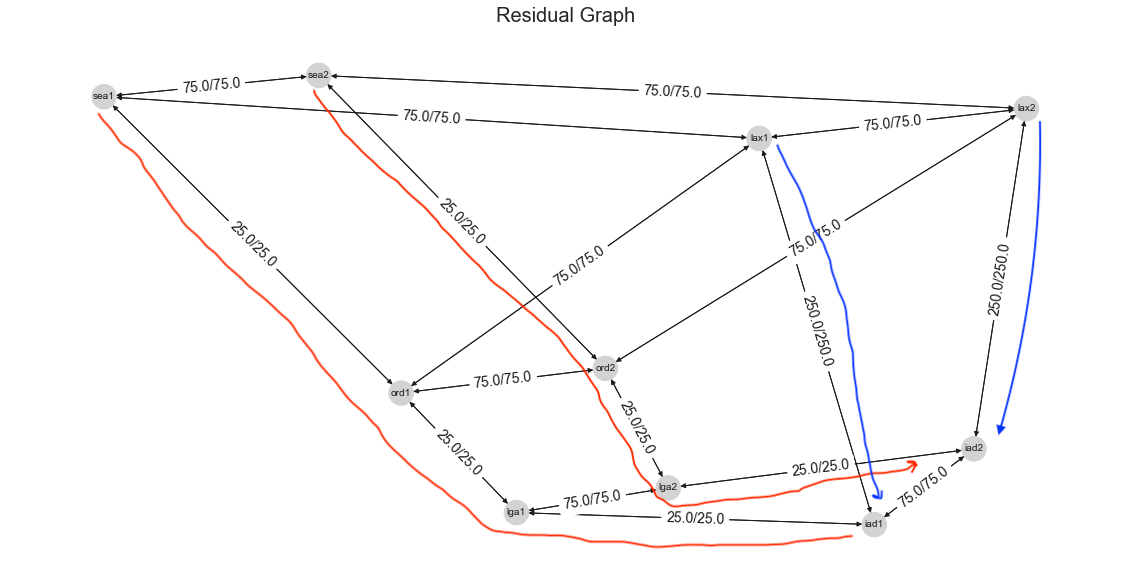
We can see the residual capacity of the links on the graph. SEA -> IAD path consists of 100G links, with 50Gbps getting routed from both SEA routers to IAD routers. This leaves us with 25Gbps on those paths. Similarity for LAX -> IAD, we have 50Gbps getting routed on each link leaving us with 250Gbps between each router pair (400 * .75 = 300.0, 300 - 50 = 250).
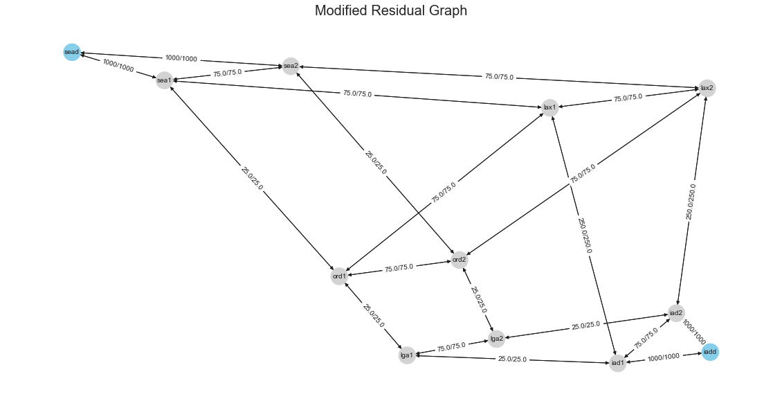
Because our primary interest is how much total traffic SEA can send to IAD, which will include both sea1 and sea2
routers, and not interested in individual routers. We will modify the residual graph by creating a dummy Source node
behind sea1 and sea2 with some large capacity between dummy node to sea1/sea2 routers. This makes sure that dummy
node edges are never a bottleneck. In our case, we will pick 1000Gbps. After adding this, our modified residual graph
looks like below:
Dinitz’s Algorithm
There are variety of algorithms available to find the Maximum Flow. Some of the well-known algorithms are like Ford-Fulkerson and Edmonds-Karp. Another algorithm for finding Max flow is Dinitz’s algorithm. It’s also known as Dinic’s algorithm because Shimon Even mispronounces the author’s name while popularizing the algorithm.
The algorithm has two main constraints which are kind of obvious to any network engineer:
Capacity Constraint: The flow on a link shouldn’t exceed its capacity. Formally $f_{uv} < c_{uv}$.
Conservation of flow: The incoming flow sent to a node is the same as an outgoing flow for transit nodes.
The algorithm creates an iterative residual network and finds a level network using Breadth-First Search(BFS). If the destination is not in the level network, it terminates; otherwise, it finds an augmenting path in the level network and repeats.
Algorithm Steps:
1) Initialize a flow with zero value, fuv=0
2) Construct a residual network N′ from that flow
3) Find the level network L using BFS; if destination is not in the level network, then break and output the flow
4) Find an augmenting path P in level network L
5) Augment the flow along the edges of path P, which will give a new residual network
6) Repeat from point 3 with new residual network
For example, we pick an initial flow of 25 from SEA to IAD on the shortest path. This will leave us with a Residual
network with edge capacities of 0 on SEA1 -> ORD1 -> LGA1-> IAD1.
example_flow = {
    ("sead", "sea1"): 25,
    ("sea1", "ord1"): 25,
    ("ord1", "lga1"): 25,
    ("lga1", "iad1"): 25,
    ("iad1", "iadd"): 25,
}
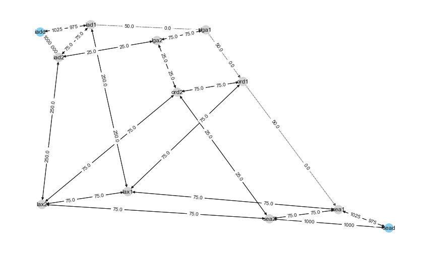
Next, we will create a level network using BFS from sead to iadd, excluding edges with 0 capacity. If the destination
was not connected to the source, we would have terminated at this step. The color in the below graph shows different levels.
We can see the edge with a minimum capacity of 75 between sead and iadd. We will use that to augment the path in the
next step.
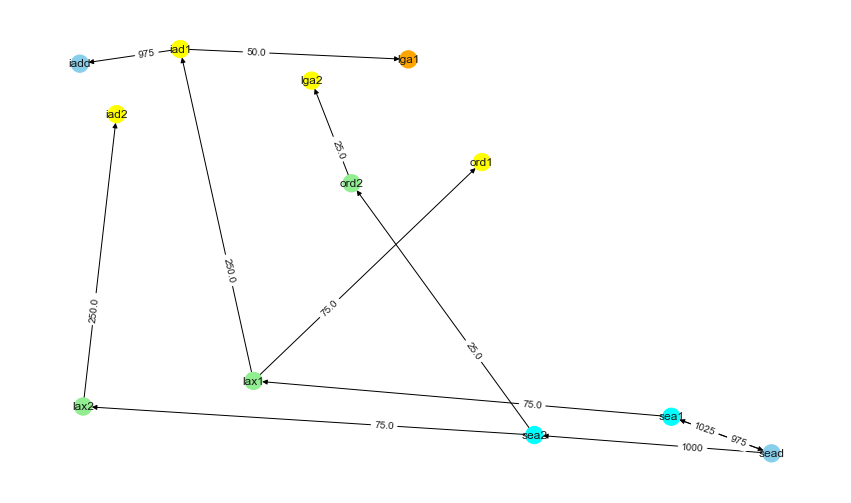
Augmented Path after applying 75Gbps on the path.
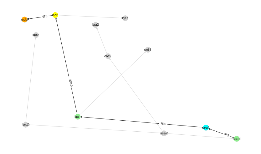
This gives us a new Residual Network where now the bandwidth between sea1 -> lax1 is now 0. So we will remove these 0 edges and create a new Level network running BFS.
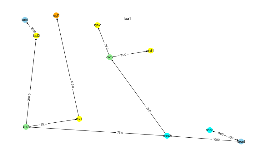
We will keep repeating these steps until Destination Node is not reachable from Source Node. I hope the above steps gave some insights into how the algorithms work.
Now let’s just do the easy way and use the algorithm to see the Max Flow for our case. It turns out that 200Gbps is the answer to our question.
from networkx.algorithms.flow import dinitz
R = dinitz(G, "sead", "iadd")
R.graph["flow_value"]

##200
The returned graph R edges have an attribute flow, which tells the flow assigned to each edge. If we plot how the
Maximum flow of 200 is distributed to various edges, we can see that SEA -> IAD flows are not on the shortest path.
They are taking SEA -> ORD -> LAX -> IAD vs taking SEA -> ORD -> LGA -> IAD.
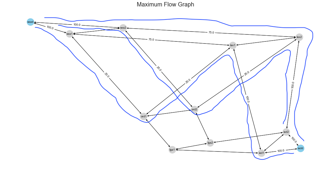
So we found how much we can send more from SEA to IAD, but the resulting flows are not assigned to the shortest path.
Minimum Cost Flow
What if we want to see the demands satisfied with the Minimum Cost path. Also, let’s extend the problem by adding another demand location from ORD -> IAD. We will assume that both ORD and SEA demands are split equally for simplicity.
Our problem now is to find the Maximum flow that the network can satisfy from both ORD and SEA to IAD.
Network Simplex
If you are familiar with linear programming, the first algorithm we learn is Simplex Method. Network Simplex is a restricted version of that applied to graphs. We will skip the details for Network simplex just because we won’t do justice without going deep into the simplex method.
Network Simplex requires us to add an attribute called demand with an integer indicating the demand. A negative demand
means that the node wants to send flow, a positive demand means that the node wants to receive flow.
Now the problem is that network simplex tries to solve whether a given demand in the network can be satisfied or not. But in our case, we don’t know the demand. So we will iteratively set a demand and keep solving for it until we get an exception that the network can not satisfy the demand anymore. This allows us to get closer to the maximum demand, which can be satisfied using the minimum cost.
# Min Cost Flow
v = 2
while True:
    v += 2
    G.add_node("sead", demand=-v/2) # Split the demand asked equally between SEA and ORD.
    G.add_node("ordd", demand=-v/2) # Split the demand asked equally between SEA and ORD.
    G.add_node("iadd", demand=v)
    try:
        minFlowCost, minFlowDict = nx.network_simplex(G)
        print(" Traffic : {:2d}\t Minimum cost :{}".format(v, minFlowCost))
    except Exception as e:
        print(" Traffic : {:2d}\t The maximum capacity of the network has been exceeded , There is no feasible flow .".format(v))
        print("\n Traffic v={:2d}: Failed to calculate minimum cost flow ({}).".format(v, str(e)))
        break

Traffic : 350	 Minimum cost :15500.0
Traffic : 352	 The maximum capacity of the network has been exceeded , There is no feasible flow.
Traffic v=352: Failed to calculate minimum cost flow (no flow satisfies all node demands).
In our case, the answer we get is 175 each from ORD/SEA or 350 aggregate to IAD. Below is the graph showing the amount of flows on each edge, satisfying both ORD/SEA demands towards IAD.
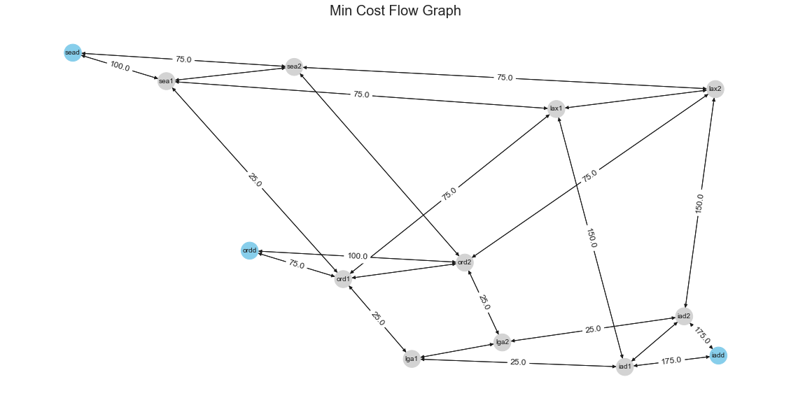
From the resulting graph, we can see an unequal split on the amount of capacity between the routers; in reality, it may not be possible to split unequal distribution of traffic to both routers. We could try first to see what happens when we route an additional 175 from SEA/ORD to IAD with 87.5 from each router. Later we can try to route 150 from SEA/ORD 75 each from both routers in the location.
model.demands.increase_absolute("sea","iad", 175) # Add 175 on top of exising 100G
model.demands.increase_absolute("ord","iad", 175) # Add 175 on top of existing 0G

print(f"{model.demands.between_regions('ord','iad').traffic}Gbps")
print(f"{model.demands.between_regions('sea','iad').traffic}Gbps")

175.0Gbps # ORD -> IAD
275.0Gbps # SEA -> IAD
model.simulate # Simulate the model again.
model.interfaces.plot_interface_utilization() # Plot the Interface Utilization
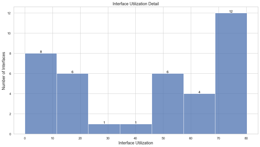
We can see some interfaces are actually surpassing our desired threshold of 75%.
for intf in list(model.interfaces.utilization()):
    print(f"{intf.name} {intf.utilization}%")

lax1-to-lax2 75.89%
sea1-to-lax1 75.89%
sea2-to-lax2 73.65%
sea1-to-ord1 73.65%
ord1-to-sea1 71.88%
sea2-to-ord2 73.65%
ord1-to-lax1 72.9%
ord2-to-lax2 80.22%
ord1-to-lga1 73.65%
ord2-to-lga2 73.65%
lga1-to-iad1 73.65%
lga2-to-iad2 73.65%
Let’s see the results for Routing 75 per router (150 aggregate vs 175 aggregate). In this case, We can see that our interface utilization is close to our target thresholds of 75%.
model.demands.decrease_absolute("sea","iad", 25)
model.demands.decrease_absolute("ord","iad", 25)

print(f"{model.demands.between_regions('ord','iad').traffic}Gbps")
print(f"{model.demands.between_regions('sea','iad').traffic}Gbps")

150.0Gbps # ORD -> IAD
250.0Gbps # SEA -> IAD

model.simulate
model.interfaces.plot_interface_utilization()
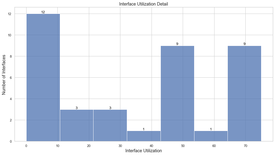
We can extend this problem where we may want to find how much more traffic can be sent on a network between various locations.
High level steps:
1) Solve it for various Source to a single Sink location.
2) Find the Maximum flow supported.
3) Route the demands in the simulation model and then get a new residual graph.
4) Repeat the steps for other sink locations.
Conclusion
In this post, we went through few algorithms that can help us find how much more bandwidth we can carry between locations on top of existing traffic. We looked at Dinitiz’s algorithm for the Maximum Flow cost without worrying about the minimum cost constraint. Then we looked at the application of the Network Simplex algorithm, which tries to satisfy all the demands with the Minimum Cost as a constraint. Then we used the results and applied them to a simulation model of an RSVP routed network to validate.
I would love to hear from anyone who has some other ways to solve problems of this nature and what methods they used.