Network Traffic Modeling Approaches
The greatest value of a picture is when it forces us to notice what we never expected to see. - John Tukey
When a city contemplates constructing a new highway or major roadway, it doesn’t simply break ground and start paving. Instead, an extensive feasibility study is conducted to evaluate various aspects including environmental impacts, traffic patterns, and potential congestion relief or creation, example: US 277 Sonora Safety Route Study, I-5 JBLM Corridor Study. These studies examine traffic patterns specific to the project area, identify existing bottlenecks, and analyze how the new infrastructure will impact the overall transportation network.
Similarly, understanding traffic patterns is fundamental to designing and operating networks, influencing decisions across all temporal and structural scales. This knowledge shapes everything from long-term, macro-level topology design to millisecond-level, micro-scale buffer allocation and tuning.
This post explores the characteristics of various traffic models using synthetic data, offering an overview of traffic patterns. We’ll generate and analyze time series data to highlight the fundamental properties of different traffic models. In a follow-up post, we will apply these insights to a practical example, examining how these traffic patterns affect the performance of Random Early Detection (RED) parameter tuning.
Also, this is a very high-level overview of the topic to provide a broader perspective. Think of this as a guided foothills tour, providing a view of the distant peaks. The climb to those distant peaks is left as an adventure for readers to explore in the future.
Statistical Distributions
Statistical Distribution Properties are fundamental in characterizing network traffic behavior. They describe the underlying probability distributions of various traffic attributes, such as packet inter-arrival times, packet sizes, flow durations, and traffic volumes.
Heavy-tailed distributions
These are probability distributions whose tails are not exponentially bounded. In network traffic, heavy-tailed distributions are often observed in phenomena like flow durations, and inter-arrival times.
- Examples include Pareto, Weibull (with shape parameter < 1), and log-normal distributions.
- They exhibit the property $P(X \gt x) \sim x^{-\alpha}$ as $x \to \infty$ where $0 \lt α \lt 2$.
- Heavy-tailed distributions can lead to high variability and extreme events in network traffic.
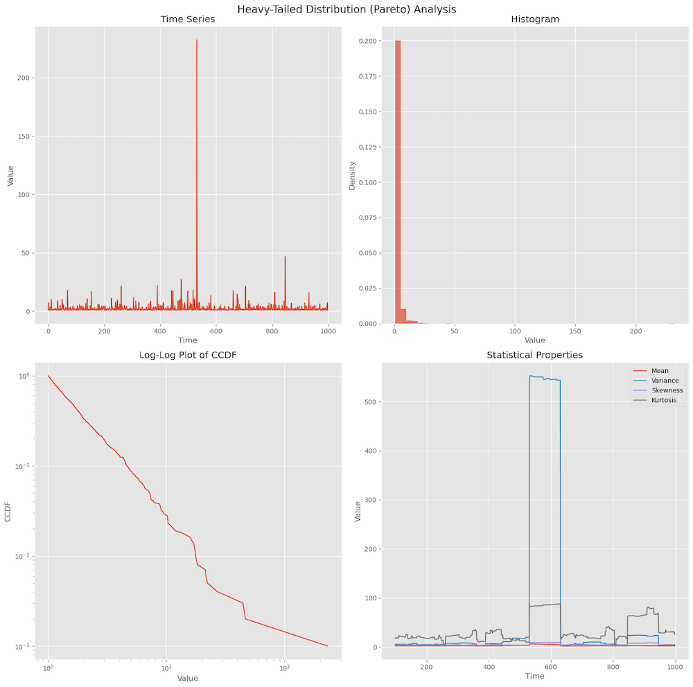
An example of a heavy-tailed distribution is below where we can see an extreme event shown by spike, and its statistical characteristics.
Service Time Distribution
This generally refers to the statistical distribution of packet sizes or the time required to process/transmit packets. Common Models are Exponential, deterministic, and more general phase-type distributions. The choice of service time distribution significantly affects queuing behavior and network performance. Service times often exhibit multi-modal distributions due to different packet size classes (e.g., ACKs, MTU-sized packets).The service time distribution impacts the queueing behavior i.e. how packets accumulate in network queues.
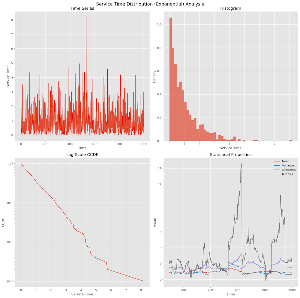
Below plot shows an example of Exponential distribution. In the time series plot we can see there are many small values with occasional large spikes. The histogram shows peal near zero and a long, gradually decreasing tail to the right.
Arrival Process
The arrival process describes the statistical nature of how packets or flows arrive at a network element. The arrival process can significantly impact on things like buffer occupation and packet loss.
Poisson Process
The classic way was to use the Poisson process. It’s a stochastic process where events (packet arrivals) occur continuously and independently at a constant average rate. The Inter-arrival times are exponentially distributed.
One of the key properties of the Poisson process is memorylessness. This means that the probability of an arrival occurring in the next time interval is independent of previous arrivals. The arrival rate $\lambda$ is constant over time, which is a very naive assumption compared to how the real traffic behaves, and that is the reason it cannot capture burstiness or correlation in real network traffic.
Many earlier research used the Poisson arrival process as an assumption for packet arrival, but it’s a very simplistic view and the real traffic patterns are more complicated.
Batch Markovian Arrival Process (BMAP)
An extension of the Poisson process that allows for batch arrivals and captures correlations and burstiness in traffic. BMAP support batch arrivals i.e. multiple packets can arrive simultaneously and is governed by an underlying Markov chain. This is suitable for modeling traffic with correlated arrivals such as bursts of packets or flows.
Self-similar Arrival Processes
Arrival processes that exhibit self-similarity, meaning their statistical properties remain consistent across different time scales. Some key properties are Long-Range Dependence i.e. significant correlations between arrivals separated by long time intervals. It exhibits a Fractal behavior i.e. the arrival process looks similar at various time scales. We can see the fractal behavior below for self-similar traffic where as we zoom in from hours to seconds, the behavior is same unlike the poisson traffic.
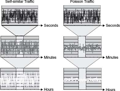
Ref: Deploying IP and MPLS QoS for Multiservice Networks
We can measure self-similarity by hurst-parameter with $0.5 \lt H \lt 1$ indicates long-range dependence. We will explore self-similarity and long-range dependence more in later section.
Markov Modulated Poisson Process (MMPP)
A Poisson process where the arrival rate is governed by a Markov chain, allowing the rate to change based on different states. This allows us to model state dependent arrival rates, where we can have different arrival rates for different states of the underlying markov chain. This is suitable to model traffic with different modes such as high and low traffic periods.
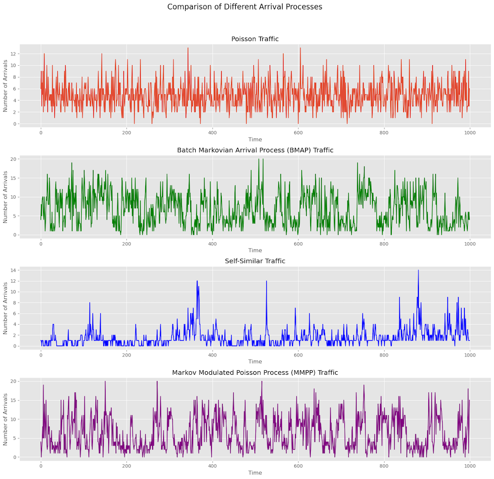
Here is a plot to show various arrival processes and how they look different. Anytime if you are modeling things like scheduling, buffer occupancy etc. the type of arrival process matters. This makes it extremely important on what assumptions one is making for the traffic pattern.
Temporal Patterns
Seasonality and Trend
Seasonality refers to regular and predictable patterns or fluctuations at specific intervals. Examples of seasonality include traffic peaking during business hours and dropping at night. Understanding seasonality helps in traffic forecasting and capacity planning.
The Trend is a long-term increase or decrease over time. The Trend indicates the general direction in which traffic patterns are moving, irrespective of short-term fluctuations or seasonal effects.
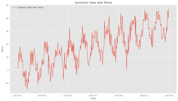
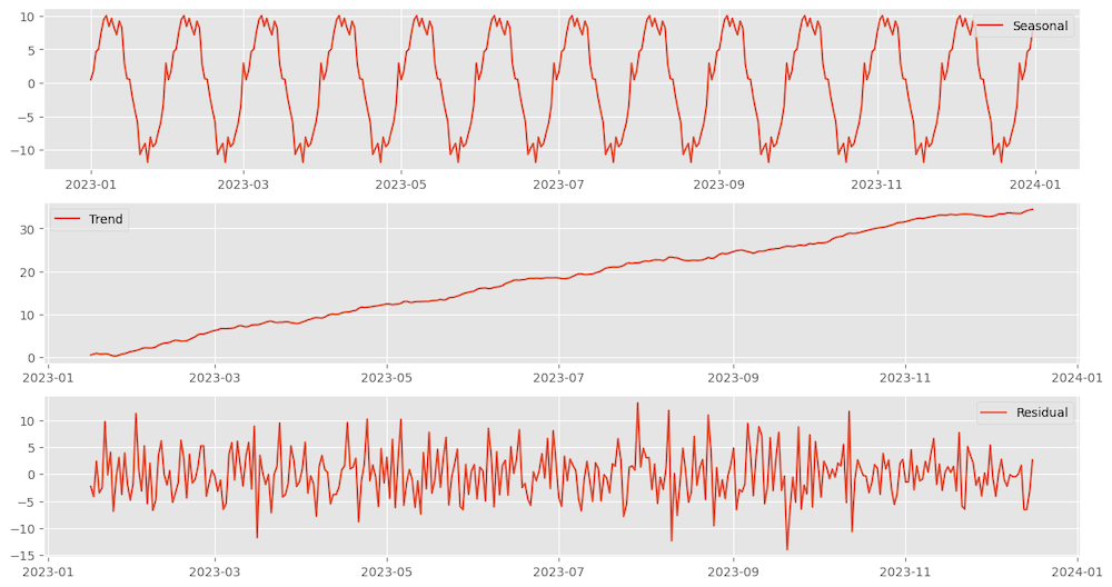
Network traffic can have both Seasonality and Trend present. One can use Seasonal Decomposition of Time Series (STL) to decompose into seasonal, Trend, and residual components. SARIMA is another classical model from econometrics that captures seasonality with ARIMA.
To extract Trend one can apply techniques like linear regression, moving average, exponential smoothing or locally weighted polynomial regression (LOESS).
Here is a time series that includes both seasonality and trend.
Decomposing the above timeseries into Seasonal, Trend and rest left as residual using STL.
ON/OFF Behavior in Network Traffic
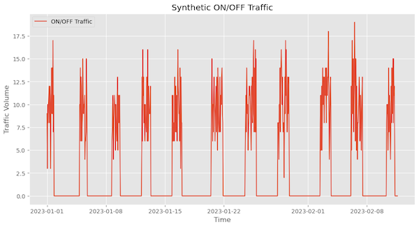
This refers to traffic patterns characterized by alternating periods of high activity (ON) and low or no activity (OFF). There is a burst of traffic during the ON periods, whereas, during the OFF periods, the traffic is minimal or nonexistent. An example of this would be traffic patterns between GPUs.
To characterize this behavior, we must understand the duration of ON and OFF periods for burstiness analysis. This can be simulated using Markov-modulated processes and decomposed using Wavelet analysis.
Here is synthetic traffic with an On/Off traffic pattern.
Scale-Related Properties
Scale related properties focuses on how traffic patterns behave and maintain consistency across different time scales.
Self-similarity and Long-Range Dependence
We already looked at this in the self-similar process section and as mentioned earlier, it’s a property where traffic patterns look similar across different time scales. This means that zooming in or out on the traffic data reveals similar structures and patterns, regardless of the time scale used.
It can be measured by Hurst Parameter which is a measure of self-similarity. Values of H ranges between 0.5 and 1.
- H = 0.5: indicates no long-term memory.
- $0.5 \lt H \lt 1$: indicates self-similarity.
- H = 1: indicates perfect self-similarity.
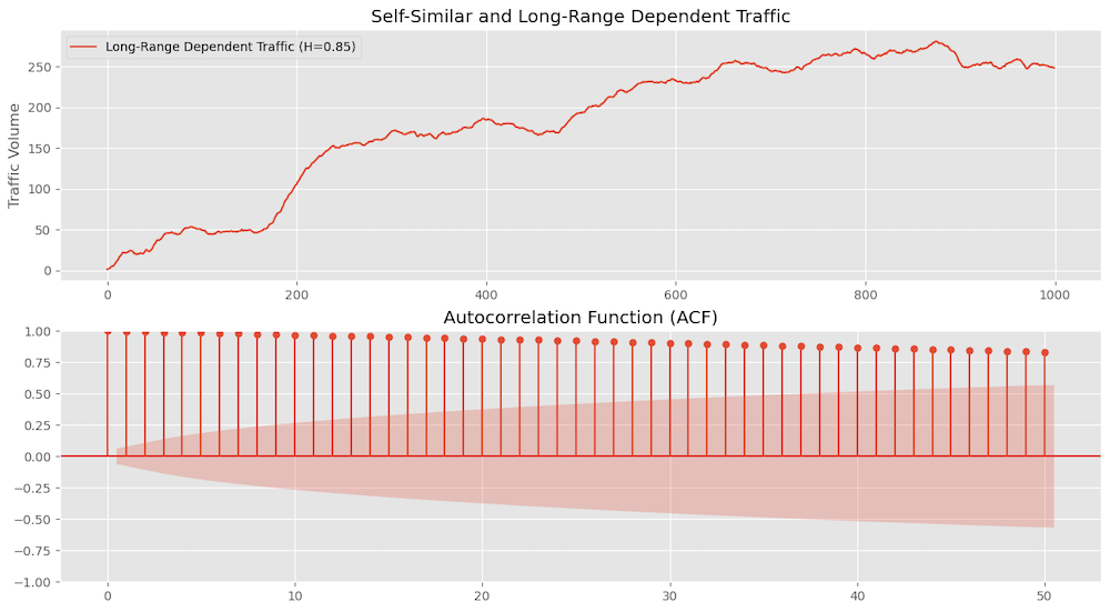
Long-range dependence (LRD) refers to significant correlations between values over long periods. We can measure this by looking at the ACF plots to see the correlation.
Here we are looking at synthetic traffic with ACF plots which shows the values decay very slowly for the lags indicating strong correlation over long periods confirming long-range dependence.
Multifractal Scaling
This is a property where traffic exhibits different scaling behaviors at different moments. This implies that the statistical properties of the traffic can vary widely, depending on the timescale and the location in the time series.
We can use Multifractal Detrended Fluctuation Analysis (MFDFA) to measure the multifractal properties of time series data.
Variability and Burstiness
Burstiness
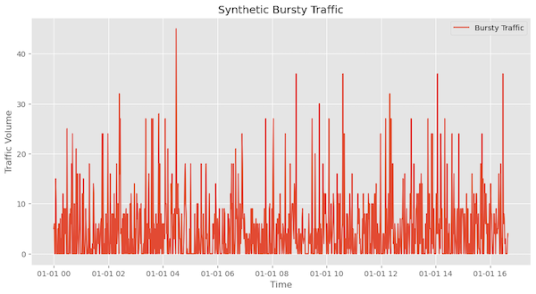
This refers to high variability in traffic over short periods. It is characterized by sudden spikes or bursts in traffic volume.
Peak to Mean Ratio
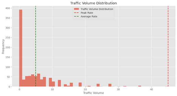
This is the difference between the peak and the average traffic rate over a period. This ratio is an important metric for understanding the extremes in traffic behavior. Below is the histogram of the above highlight the peak and average rate of traffic observed.
Variability (Coefficient of Variation)
The Coefficient of Variation (CV) is a measure of relative variability. It is defined as the ratio of the standard deviation to the mean of the traffic volume.
Correlation and Dependency
Autocorrelation and Partial Autocorrelation
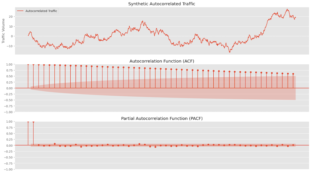
Autocorrelation is the correlation of a signal with a delayed copy of itself as a function of delay. In other words, it measures how similar the observations are between time series points separated by a given time lag. The autocorrelation function (ACF) gives us the correlation between any two values of the same variable at times $t_{i}$ and $t_{j}$. We can also use PACF to measure the correlation between an observation $Y_{t}$ and $Y_{t-k}$ after removing the effects of all the intermediate observations $Y_{t-1}, Y_{t-2}, …, Y_{t-k+1}$.
Below we have an auto-correlated series and the ACF plot shows that values start at 1 for lag 0 and remain significantly positive for many lags indicating strong autocorrelation. The slow decay of the ACF values indicates that the traffic has a strong autocorrelation structure, meaning that traffic volumes at one time point are highly influenced by previous lags.
The sharp decline in the PACF values after the first few lags indicates that the traffic is primarily influenced by the most recent past values. This suggests that while there is strong autocorrelation in the short term, the direct influence of traffic volumes diminishes quickly with increasing lag.
Random Walk
A random walk is a stochastic process that describes a path consisting of a succession of random steps. It is a fundamental concept in probability and is used to model various phenomena in fields such as physics, finance, and network theory.
Some main properties are:
- The path is formed by a series of steps, where each step is determined by a random process.
- Each step is independent of the previous steps.
- The statistical properties of the steps do not change over time (Stationarity).
Examples:
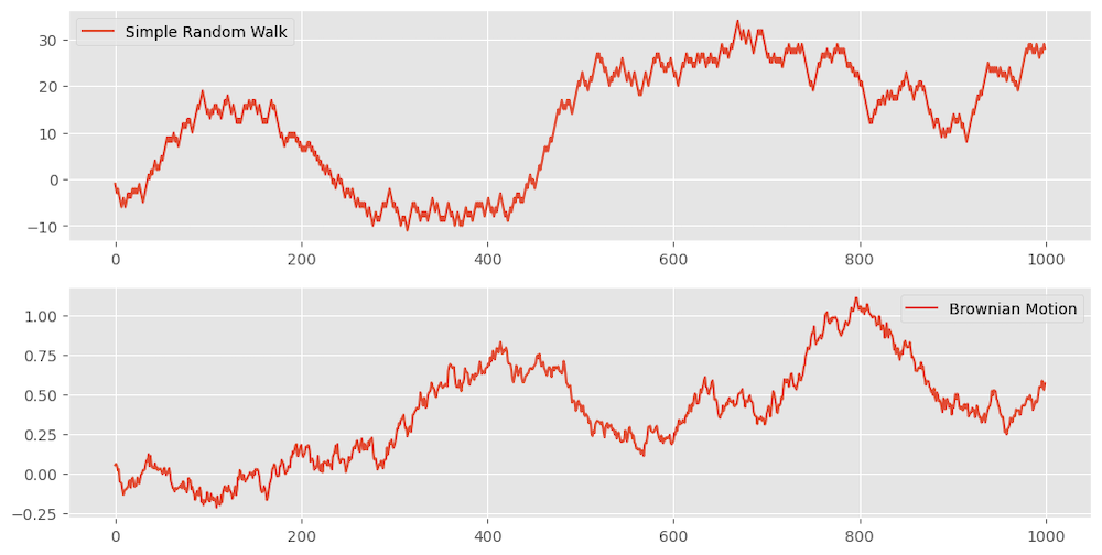
Simple Random Walk: A process where each step is equally likely to move up or down by a fixed amount. This can be given by $X_{t} = X_{t-1} + \epsilon_{t}$. where $\epsilon_{t}$ is a random variable.
Brownian Motion: A continuous-time random walk where the steps follow a normal distribution. This can be given by $X(t) = X(0) + \int_{0}^{t}\sigma dW(s)$ where $W(s)$ is a wiener process and $\sigma$ is the volatility.
Here is a synthetic simple random walk and brownian motion example:
Stationarity and Time-Invariance
Stationarity
A time series is said to be stationary if its statistical properties, such as mean, variance, and autocorrelation, do not change over time. This implies that the process generating the data remains constant over time.
Types of Stationarity:
-
Strict Stationarity: The joint distribution of any set of observations is invariant under time shifts. This is a very strong condition and is rarely met in practice.
-
Weak Stationarity (Second-Order Stationarity): Only the first two moments (mean and variance) and the autocorrelation structure are invariant under time shifts. This is more commonly used in practical applications.
A time series is said to be non-stationary if its statistical properties change over time. This includes changes in mean, variance, autocorrelation, and the presence of trends or seasonal patterns.
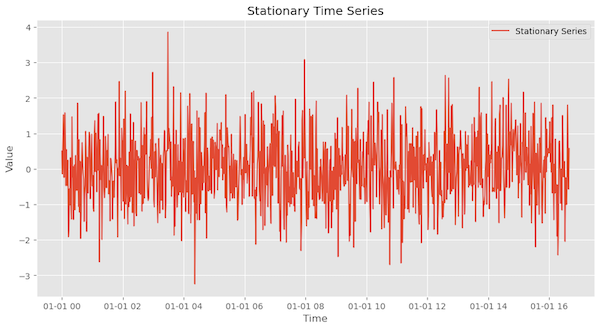
This is an example of stationary time series, which we can see the mean and variance seems to be stable over time.
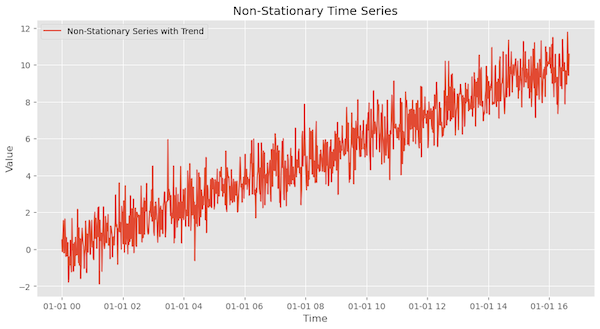
This is an example of Non-Stationary time series as it has trend which means the mean is not constant over time.
Conclusion
We looked at several foundational properties of a network traffic that are essential to understand. These include temporal patterns like seasonality and trends, scale-related behaviors such as self-similarity and long-range dependence, and statistical distribution characteristics. Each property uniquely influences network performance. For example, buffer sizing and packet drops will vary depending on the traffic’s burstiness and arrival patterns.
In the next post, we will simulate a Random Early Detection (RED) process and explore how different parameters impact network performance based on various traffic characteristics.