Introduction

A system is robust if the failure of some components doesn’t affect its function. As network engineers, we face various types of network failures like link, node failures all the time.

Generally, we use various Network modeling tools like Cariden(WAE), WANDL, etc. to model failures and see how the network reacts under a given failure condition. The components which are in play are:

1. Type and Number of failures. Type: Link, Node. Number of Failures: Single or Double.
2. Routing protocols running on top of the network and there reaction to the failure. Example: RSVP-TE, Pure IGP, SR-TE etc.
3. Network flows and their volume.
4. Network Topology.

In this blog post, we will focus purely on #4 Network topology and certain characteristics of topology, which may make them more robust than other topologies.

Key Idea

The network topology may have some critical nodes. If we can identify them and take them out of the service, they will significantly impact the functionality of the network. For example, in the case of a Hub and Spoke topology, if a Hub is out of service, it affects all the spokes vs. a spoke out of service. We can make this hub and spoke topology more robust if we have multiple hubs, which means we don’t have a single node that is the most critical.

So this brings the question: How do we identify important nodes in a topology? This brings to our next topic i.e. Centrality measures.

Centrality Measures

The importance of a node or link is identified by computing its centrality. The higher the score, the more critical is the node. There are several ways to compute Centrality:

1. Degree
2. Closeness
3. Betweenness

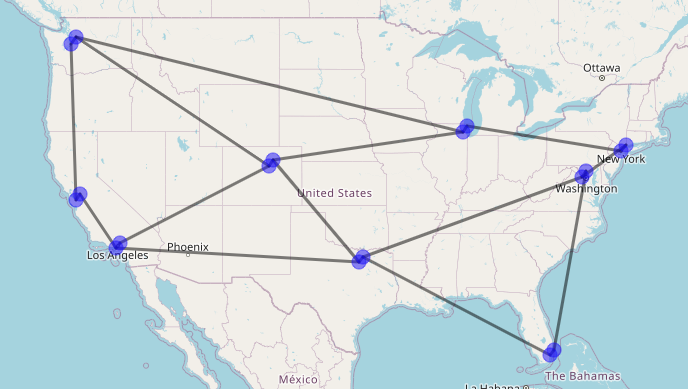
For our example, we will follow the below sample topology. The graph computed is a directed graph with weight=1. In reality, weights will be different based on the IGP cost representing latency, but I have skipped that detail here.

Degree

As we know, the degree of a node is the number of nodes it’s connected to. The intuition here is that if a node is connected to a lot of other nodes, then it must be an important node.

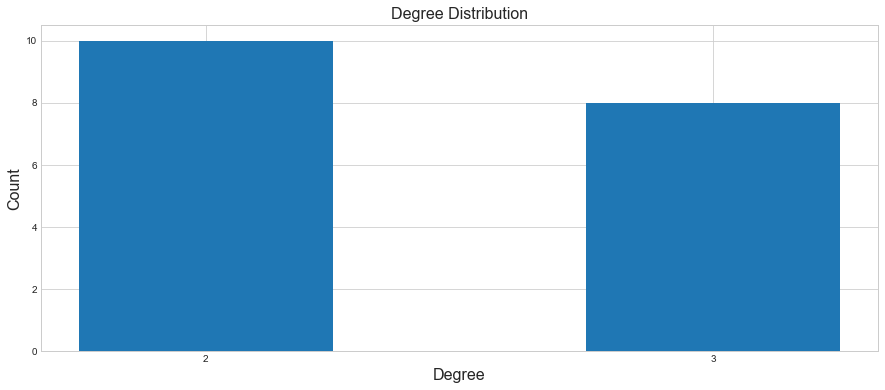
If we look at the degree distribution of our sample topology, there are 10 nodes with degree 2 and 8 nodes with degree 3. Below is a histogram of that.

degree_sequence = [G.degree(n) for n in G.nodes]
from collections import Counter
degree_counts = Counter(degree_sequence)

fig, ax = plt.subplots(figsize=(15,6))
plt.title('Degree Distribution', fontsize=16)
plt.xlabel('Degree', fontsize=16)
plt.ylabel('Count', fontsize=16)
plt.bar(range(len(degree_counts)), list(degree_counts.values()), width=.5,align='center',)
_ = plt.xticks(range(len(degree_counts)), list(degree_counts.keys()))

Closeness

Another way to measure the centrality of a node is by determining how close it is to other nodes. This can be computed by summing the distances from the node to all others. If the distances are short on average, their sum is a smaller number, and we can say that the node has high centrality.

Closeness centrality is defined by

where $l_{ij}$ is the distance from i to j and the sum runs over all the nodes.

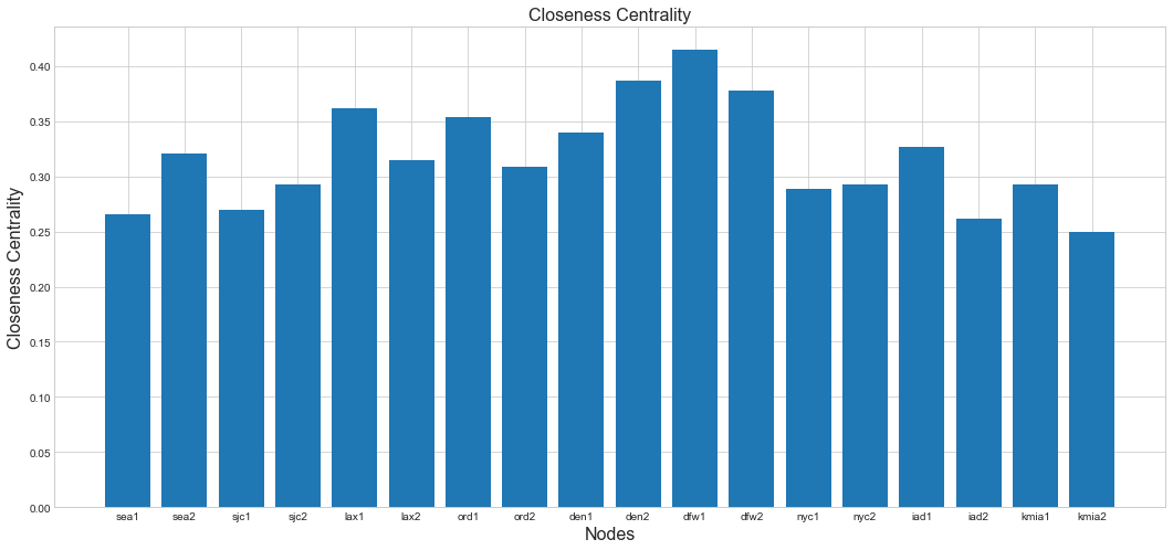
If we look at the Closeness centrality of our sample topology, seems like DFW1, DFW2 and DEN2 are the top three. Below is a histogram of that.

Betweenness

The general idea here is that a node is more central, the more often its involved. The simplest way to calculate is to calculate the shortest path from each node to every other node. The centrality is computed by counting how many times a node shows up in those shortest paths. The higher the count of node, the more traffic it controls.

bc = nx.betweenness_centrality(G)
fig, ax = plt.subplots(figsize=(18,8))
plt.title('Betweenness Centrality', fontsize=16)
plt.xlabel('Nodes', fontsize=16)
plt.ylabel('Betweenness Centrality', fontsize=16)
plt.bar(range(len(bc)), list(bc.values()),align='center')
_ = plt.xticks(range(len(bc)), list(bc.keys()))

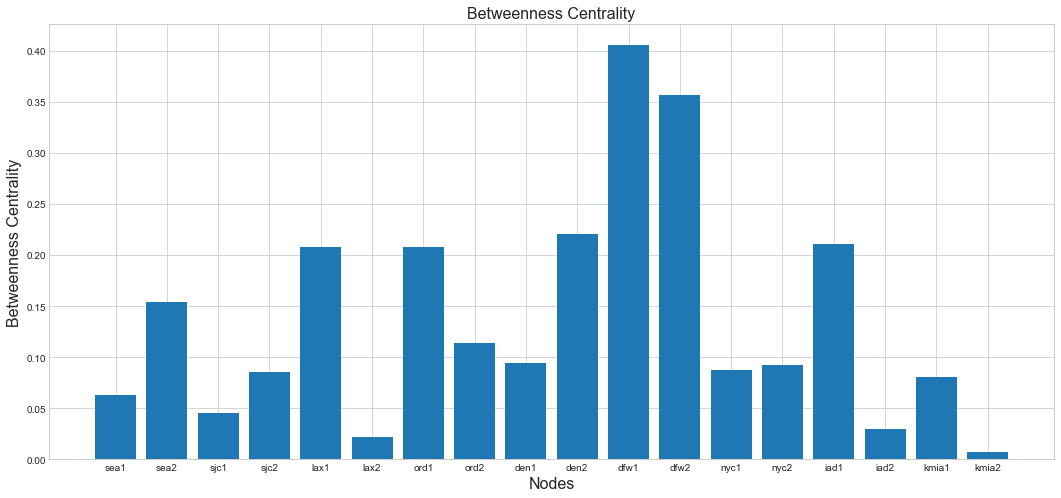
In case of betweenness centrality, dfw1 and dfw2 stand out the most.

Robustness

The standard way to check the robustness is by seeing how connected the graph is when we start removing the nodes. Removal of nodes can be either random or systematic. To estimate the disruption following a node removal, we compute the relative size of the giant component i.e. ratio of the number of nodes in the giant component to the number of nodes initially present in the network.

Assuming a connected graph, when we start initially, the whole graph is one giant component. If removing a subset of nodes does not break the graph into two disconnected graphs, then the proportion of the nodes in the giant component gets reduced by the number of removed nodes. If, however, the node removal breaks the network into two or more connected graphs, the size of the giant component may drop substantially.

Testing the robustness of the sample topology by removing 2 nodes with highest degree.

N = G.number_of_nodes()   # No. of nodes are 18
number_of_steps = 8       # How many iterations we want to perform.
M = N // number_of_steps  # M = 2 here. This means we will take two nodes at a time.

num_nodes_removed = range(0, N, M) # Number of nodes to be removed. 
C = G.copy()                       # Make a copy of the graph
targeted_attack_core_proportions = [] #list to capture the results
for nodes_removed in num_nodes_removed: #Let's iterate over the nodes
    # Measure the relative size of the network core
    core = next(nx.connected_components(C)) #Compute the connected component
    core_proportion = len(core) / N         #Core_proportion 
    targeted_attack_core_proportions.append(core_proportion)
    
    # If there are more than M nodes, select top M nodes and remove them
    if C.number_of_nodes() > M:          #if the number of nodes left is greater than 2
        nodes_sorted_by_degree = sorted(C.nodes, key=C.degree, reverse=True) #Get the highest degree nodes
        nodes_to_remove = nodes_sorted_by_degree[:M] # Get two nodes
        C.remove_nodes_from(nodes_to_remove)         # Remove the nodes

fig, ax = plt.subplots(figsize=(15,6))
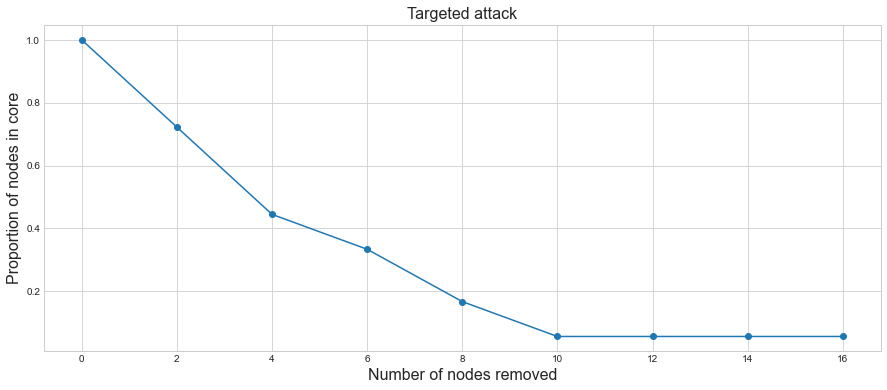
plt.title('Targeted attack', fontsize=16)
plt.xlabel('Number of nodes removed',fontsize=16)
plt.ylabel('Proportion of nodes in core',fontsize=16)
plt.plot(num_nodes_removed, targeted_attack_core_proportions, marker='o')

What we observe is that once we removed two nodes in the first iteration, the proportion of the nodes left in the giant are around 72%

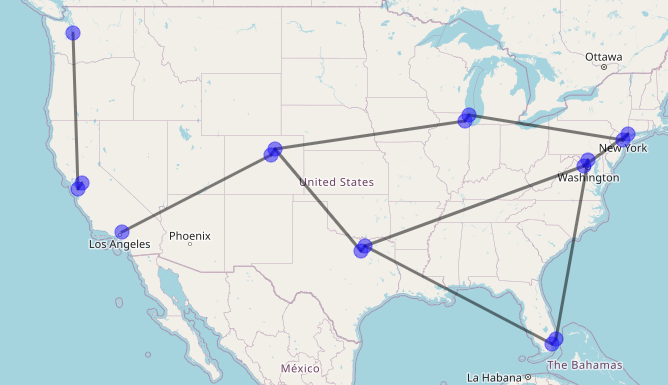
After removing sea2 and lax1 we see that the left side of the graph is isolated.

Summary

We looked at various centrality measures and then looked at application of degree centrality to check the robustness of the graph.

In large networks, it is necessary to use statistical tools to analyze the global features of the network. These tools can also help in comparing various topologies. I hope you get something useful out of this post.