In a previous post, I discussed how Maximum Flow problems can be used for network optimization. We focused on a scenario where demands were already routed in the network, and our objective was to determine the maximum demand that could be handled between a given source and a destination metro. We solved this problem by calculating the residual bandwidth for the graph, creating fake demand nodes for each metro with high-capacity edges to avoid them being bottlenecks, and applying Dinic’s algorithm between the source and the destination metro. This is also called a Single Commodity Flow Problem.

We then extended the problem to consider two metros sending traffic to the same destination sink and used the Network Simplex algorithm to determine the maximum traffic the network could accommodate. This is also known as a Multi Commodity Flow Problem. Finally, we validated our findings by routing the results through a network model.

In this post, we will discuss another constraint-based problem called Minimum Maximum Link Utilization (MMLU). The primary goal of MMLU is to route traffic demands in a network to minimize the maximum link utilization. In other words, we aim to distribute the traffic evenly across the network links to avoid over-utilizing any particular link. This approach is useful when dealing with traffic demands that are not latency-sensitive, and the paths taken do not necessarily need to be the shortest. Instead, the focus is on spreading the traffic evenly across the network to ensure no single link becomes a bottleneck.

By addressing the MMLU problem, we can optimize network performance, improve overall network utilization, and reduce the risk of congestion or link failures due to excessive utilization.

Problem Setup

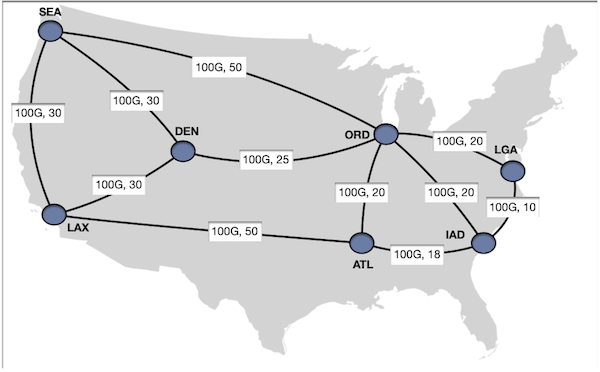
We will use this trivial topology as an example. All the links have a 100G capacity, and the respective link cost is listed in the picture.

We will start with a trivial case that we have sea, lax, ord, den, atl all sending $\text{20 Gbps}$ to iad.

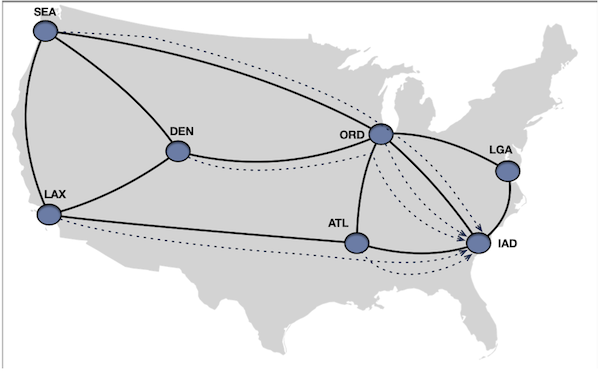
If we route these demands just via shortest paths, highlighted below, we see that ord -> iad link is getting used by demands routing from sea, den, ord to iad and atl -> iad link is getting used by demands routing from lax, atl to iad.

Here is the path for each demand the shortest path costs for each paths.

So the ord -> iad $\text{100 Gbps}$ link is carrying a total of $\text{60 Gbps}$ i.e. 60% utilized and atl -> iad link is carrying a total of $40 \hspace{2pt} Gbps$ i.e. 40% utilized, while lga -> iad link being 0% utilized. In this case, we have the maximum link utilization of 60% and our goal here is can we do better and minimize the maximum link utilization. In order to appreciate the problem, try solving this in your head before you read it further and see if your answer matches at the end. If you solved this problem, then try solving for this traffic demand.

Metrics to Measure Maximum Link Utilization

Before we delve into solving the problem, it would be beneficial to develop a scoring mechanism that allows us to measure the overall quality of the solution. This score can be used to compare different solutions and determine if one is superior to the others.

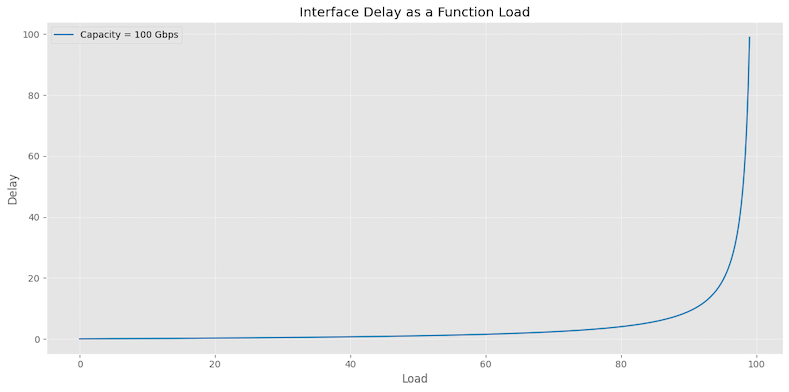
One potential approach to calculate this score is by computing the ratio $\frac{\text{Traffic Load}}{\text{Interface Capacity} - \text{Traffic Load}}$ for each interface. This ratio is derived from the queueing delay result of the M/M/1 model and represents a version of the classical hockey stick diagram, as plotted below. The relationship between the traffic load and the delay is nonlinear.

To obtain an aggregate delay measure, we sum the ratios $\frac{\text{Traffic Load}}{\text{Interface Capacity} - \text{Traffic Load}}$ for all interfaces, resulting in a total delay value, denoted as $\text{Total Delay}$. Then, we calculate a network-level average delay score by dividing the total delay by the total bandwidth carried by the interfaces, expressed as $\frac{\text{Total Delay}}{\text{Total BW}} * 1000$.

This scoring mechanism provides a quantitative measure of the overall solution quality, taking into account the traffic load, interface capacity, and total bandwidth. By comparing the scores of different solutions, we can determine which one achieves a lower average delay and, consequently, a better performance in terms of network utilization and congestion.

Below is the mathematical formulation.

Let:

• $D$ be the set of demands.
• $I$ is the set of interfaces.
• $T_{d}$ be the traffic associated with demand d.
• $C_{i}$ be the capacity of interface i.
• $L_{i}$ be the traffic load on interface i.
• $\text{Total BW}$ be the total bandwidth being carried by all demands.
• $\text{Total Delay}$ be the sum of delays across all utilized interfaces.

Procedure:

1. Calculate Total Bandwidth: $\text{Total BW} = \sum_{d \in D}T_{d}$
2. Calculate Total Delay: For each unique interface $i$ , calculate the delay if $L_{i} < C_{i}$: $\text{Total delay} = \sum_{i \in I}\frac{L_{i}}{C_{i}-L_{i}}$
3. Calculate Average Delay: If $\text{Total BW} > 0$, calculate the average delay as: $\text{avg_delay} = \frac{\text{Total Delay}}{\text{Total Bw}} * 1000$ else, set $\text{avg_delay=0}$.

Calculating this score for the paths routed over the shortest paths, we get 29.1

Links
sea->ord: 20/(100-20) = .25  
den->ord: 20/(100-20) = .25
lax->atl: 20/(100-20) = .25
ord->iad: 60/(100-60) = 1.50 # Higher Score for Higher Load.
atl->iad: 40/(100-40) = 0.66

Sum of al the links = 2.91
Total BW from all the demands = 100
Avg. Delay Score = 0.0291 x 1000 = 29.1

Minimizing Maximum Link Utilization

There are different ways to approach the problem of Min-Max Link Utilization. One possible method is to develop a heuristic algorithm that explores various paths for each source-destination demand pair. The algorithm would select a path out of many for each demand pair. Then, a metric that was previously derived for the overall solution would be calculated. This process would be repeated for different combinations. Since each demand pair can have multiple paths where the demand can be allocated, the algorithm would choose the combination that results in the lowest overall score. This method may not guarantee an optimal solution, but it can provide an approximation that is close to the optimal solution.

Another option is to formulate the Min-Max Link Utilization problem as a Linear Program (LP) and solve it using a LP solver. If you don’t know what a Linear Program is, This article Linear Programming and Disjoint Path Routing goes through the basics of a linear program. In essence, you have an Objective function which you want to minimize or maximize, you have some decision variables associated with the problem, and certain constraints which you want to meet. Once the problem is formulated, we use a LP solver to solve that problem.

LP Formulation

Objective Function:

So the objective we have in hand is to minimize the maximum utilization across all links in the network.

Subject to:

Flow Variables:

For each link $(i,j)$ in the network graph $G$, we have a flow variable representing the amount of traffic flow on that link. This tracks the flow for that given link.

This scary looking notation in simple words is that the flow variable for a given link $(i,j)$ is either 0 or greater, for all (expressed as $\forall$) links which are part of graph $G$.

Max Util Variable:

We put a constraint that Maximum Utilization can be greater or equal to 0.

Flow Conservation Constraints for each node:

For network flow problems with LP formulation, we generally have flow conservation constraint which says, except the source and destination nodes of the demands, the amount of traffic entering is equal to the traffic leaving the node for a transit node.

The above equation $E$ is the set of edges, $f_{i,j}$ is the flow on each edge $(i,j)$ and $n$ is the transit node. $b_{n}$ is the net flow at node $n$ (+ve for sources, negative for sinks, and zero for transit nodes).

Capacity and Utilization Constraints:

For each link, the flow must not exceed the link’s capacity, and the link’s utilization must not exceed the $U$ variable.

Where $C_{i,j}$ is the capacity of edge $(i,j)$. This make sense as we don’t want the flow on a link to be more than the capacity of the link.

Utilization constraint for each edge $(i,j)$ says that the $\frac{\text{Traffic On Link}}{\text{Capacity On Link}} \le \text{Maximum Link Utilization}$.

We convert this constraint to $f_{ij} \le U \times C_{ij}$.

Demand constraints for each demand pair (s,t,d):

For source $s$ of the demand:

For destination $t$ of the demand:

Here is the code implementation of the above problem. We are using pulp for linear programming and CBC MILP Solver. There are other solvers including commercial solvers available as well.

demands = [
    ('sea', 'iad', 20),
    ('lax', 'iad', 20),
    ('ord', 'iad', 20),
    ('den', 'iad', 20),
    ('atl', 'iad', 20),
]
# Define the linear programming problem
prob = LpProblem("Min_Max_Link_Utilization_Extended", LpMinimize)

# Variables for the flow on each edge
flow_vars = LpVariable.dicts("Flow", [(i, j) for i, j in G.edges()], 0)

# Variable for the maximum utilization
max_util = LpVariable("MaxUtil", lowBound=0)

# Objective function
prob += max_util, "Minimize the maximum link utilization"

# Flow conservation constraints
net_flow = {node: 0 for node in G.nodes()}
for src, tgt, amt in demands:
    net_flow[src] += amt
    net_flow[tgt] -= amt

for node in G.nodes():
    prob += (
        lpSum(flow_vars[i,j] for i, j in G.edges() if i == node) - 
        lpSum(flow_vars[j,i] for j, i in G.edges() if i == node)
    ) == net_flow[node], "Flow conservation for node {}".format(node)

# Capacity and utilization constraints
for i, j in G.edges():
    capacity = G[i][j][0]['capacity']
    prob += flow_vars[i, j] <= capacity, "Capacity constraint for edge ({}, {})".format(i, j)
    prob += flow_vars[i, j] <= capacity * max_util, "Utilization constraint for edge ({}, {})".format(i, j)

# Solve the problem
prob.solve()

# Print the results
print("Status:", LpStatus[prob.status])
print("Maximum link utilization:", value(max_util))
for var in prob.variables():
    if "Flow" in var.name:
        print(f"{var.name}: {var.varValue}")


Status: Optimal
Maximum link utilization: 0.33333333
Flow_('atl',_'atl_dmd'): 0.0
Flow_('atl',_'iad'): 33.333333
Flow_('atl',_'lax'): 0.0
Flow_('atl',_'ord'): 0.0
Flow_('atl_dmd',_'atl'): 0.0
Flow_('den',_'den_dmd'): 0.0
Flow_('den',_'lax'): 0.0
Flow_('den',_'ord'): 20.0
Flow_('den',_'sea'): 0.0
Flow_('den_dmd',_'den'): 0.0
Flow_('iad',_'atl'): 0.0
Flow_('iad',_'iad_dmd'): 0.0
Flow_('iad',_'lga'): 0.0
Flow_('iad',_'ord'): 0.0
Flow_('iad_dmd',_'iad'): 0.0
Flow_('lax',_'atl'): 13.333333
Flow_('lax',_'den'): 0.0
Flow_('lax',_'lax_dmd'): 0.0
Flow_('lax',_'sea'): 6.6666667
Flow_('lax_dmd',_'lax'): 0.0
Flow_('lga',_'iad'): 33.333333
Flow_('lga',_'lga_dmd'): 0.0
Flow_('lga',_'ord'): 0.0
Flow_('lga_dmd',_'lga'): 0.0
Flow_('ord',_'atl'): 0.0
Flow_('ord',_'den'): 0.0
Flow_('ord',_'iad'): 33.333333
Flow_('ord',_'lga'): 33.333333
Flow_('ord',_'ord_dmd'): 0.0
Flow_('ord',_'sea'): 0.0
Flow_('ord_dmd',_'ord'): 0.0
Flow_('sea',_'den'): 0.0
Flow_('sea',_'lax'): 0.0
Flow_('sea',_'ord'): 26.666667
Flow_('sea',_'sea_dmd'): 0.0
Flow_('sea_dmd',_'sea'): 0.0

The solution obtained from the linear programming solver shows that we can achieve a maximum link utilization of 33.33% across all links in the network. The solver provides us with the optimal flow allocation, which tells us how much traffic each interface should carry to minimize the maximum link utilization. However, the solution lacks a crucial piece of information, which is the specific contribution of each source-destination demand pair to the flow on each interface.

This missing information creates a challenge when it comes to implementing the solution in practice. For instance, if we want to program our network using explicit Traffic Engineering (TE) tunnels, we need to know precisely how much traffic from each source-destination pair should be allocated to each tunnel. Without this detailed information, it becomes challenging to configure the TE tunnels effectively and ensure that the desired traffic distribution is achieved.

Modified LP Formulation

In order to track which demand is contributing how much for a given interface, we will create flow variables per demand. In that way we can keep track of the demands. Let’s look at the modified LP formulation

Objective Function:

Flow Conservation for Each Demand:

For each demand $d=(s_{d},t_{d},A_{d})$ and each node $n \in V$,

• $s_{d}$ is the source node of demand $d$.
• $t_{d}$ is the target (destination) node of demand $d$.
• $A_{d}$ is the amount of demand (flow) that needs to be routed from $s_{d}$ to $t_{d}$.

We define $F_{sd,td,i,j}$ as the flow variable representing the flow of demand $d$ through edge $(i,j)$.

For Non-Source and Non-Destination Nodes:

For any intermediate node $n$ (i.e., a node that is neither the source nor the destination of the demand), the total incoming flow must equal the total outgoing flow.

The sum of flows on all edges leading into node $n$ minus the sum of flows on all edges leading out of node $n$ must be zero. This ensures that whatever flow enters the node also leaves it, maintaining flow continuity.

For the Source Node ($s_{d}$):

For the source node of demand $d$, the total outgoing flow minus any incoming flow must equal the demand amount $A_{d}$.

The net flow out of the source node must match the demand amount. This ensures the demand is fully routed out of the source.

For the Destination Node ($t_{d}$):

For the destination node of demand $d$, the total incoming flow minus any outgoing flow must equal the demand amount $A_{d}$.

The net flow into the destination node must match the demand amount. This ensures the demand is fully delivered to the destination.

Capacity Constraints for Each Edge:

For each edge $(i,j) \in E$, the sum of flows for all demands through this edge must not exceed its capacity.

Utilization Constraints for Each Edge:

For each edge $(i,j) \in E$, the sum of flows for all demands through this edge, divided by the edge’s capacity, must not exceed the maximum utilization $U$.

We will modify this constraint to

Here is the modified code implementation

# More complex demands between pairs (source, target, demand_value)
demands = [
    ('sea', 'iad', 20),
    ('lax', 'iad', 20),
    ('ord', 'iad', 20),
    ('den', 'iad', 20),
    ('atl', 'iad', 20),
]

# Define the linear programming problem
prob = LpProblem("Min_Max_Link_Utilization_Extended", LpMinimize)

# Variables for the flow on each edge for each demand
flow_vars = LpVariable.dicts("Flow", [(src, tgt, i, j) for src, tgt, _ in demands for i, j in G.edges()], 0)

# Variable for the maximum utilization
max_util = LpVariable("MaxUtil", lowBound=0)

# Objective function
prob += max_util, "Minimize the maximum link utilization"

# Flow conservation constraints
for src, tgt, amt in demands:
    for node in G.nodes():
        if node == src:
            prob += lpSum(flow_vars[src, tgt, node, j] for _, j in G.edges(node)) - lpSum(flow_vars[src, tgt, i, node] for i, _ in G.in_edges(node)) == amt
        elif node == tgt:
            prob += lpSum(flow_vars[src, tgt, i, node] for i, _ in G.in_edges(node)) - lpSum(flow_vars[src, tgt, node, j] for _, j in G.edges(node)) == amt
        else:
            prob += lpSum(flow_vars[src, tgt, node, j] for _, j in G.edges(node)) - lpSum(flow_vars[src, tgt, i, node] for i, _ in G.in_edges(node)) == 0

# Capacity and utilization constraints
for i, j in G.edges():
    capacity = G[i][j][0]['capacity']
    prob += lpSum(flow_vars[src, tgt, i, j] for src, tgt, _ in demands) <= capacity
    prob += lpSum(flow_vars[src, tgt, i, j] for src, tgt, _ in demands) <= capacity * max_util

prob.solve()

# Print the results
print("Status:", LpStatus[prob.status])
print("Maximum link utilization:", value(max_util))


if LpStatus[prob.status] == "Optimal":
    print("Maximum link utilization:", value(max_util))
    for src, tgt, _ in demands:
        print(f"Demand from {src} to {tgt}:")
        for i, j in G.edges():
            if value(flow_vars[src, tgt, i, j]) > 0:
                print(f"  Flow on edge ({i}, {j}): {value(flow_vars[src, tgt, i, j])}")
else:
    print("Problem is infeasible or no optimal solution found.")

Status: Optimal
Maximum link utilization: 0.33333333
Demand from sea to iad:
  Flow on edge (sea, ord): 20.0
  Flow on edge (ord, lga): 20.0
  Flow on edge (lga, iad): 20.0
Demand from lax to iad:
  Flow on edge (lax, atl): 20.0
  Flow on edge (atl, iad): 20.0
Demand from ord to iad:
  Flow on edge (ord, iad): 20.0
Demand from den to iad:
  Flow on edge (ord, lga): 13.333333
  Flow on edge (ord, iad): 6.6666667
  Flow on edge (den, ord): 20.0
  Flow on edge (lga, iad): 13.333333
Demand from atl to iad:
  Flow on edge (ord, iad): 6.6666667
  Flow on edge (atl, ord): 6.6666667
  Flow on edge (atl, iad): 13.333333

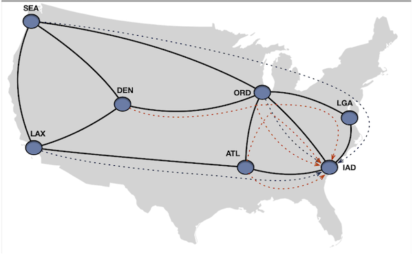
So this looks better now. I know exactly which demand is routed via which links. If we calculate the score for this solution, we get $24.2$ which is lower than previous score $29.1$ and hence better. Looking back on our graph what we see is

• sea -> iad is routed via lga.
• den -> iad is split into two paths, one on direct path and other via lga.
• atl -> iad is split into two paths, one on direct path and other via ord.
• ord -> iad is routed on the direct path.

Because some of the demands like den -> iad is split into two paths, i..e den-> ord -> lga -> iad path carrying $13.33$ and den -> ord -> iad carrying $6.66$ of the total $20$. So to program the traffic engineering tunnels, we would need some sort of weighted ECMP support. If we are using SR-TE, then each Path-List can have different weights to carry the appropriate amount of traffic.

Solving for the bigger demand set

The answer we get is $60$%. Is it the most optimal or not is left as an exercise for the reader.

Maximum link utilization: 0.6
Demand from sea to iad:
  Flow on edge (sea, ord): 20.0
  Flow on edge (ord, iad): 20.0
Demand from lax to iad:
  Flow on edge (lax, atl): 20.0
  Flow on edge (atl, iad): 20.0
Demand from ord to iad:
  Flow on edge (ord, iad): 20.0
Demand from den to iad:
  Flow on edge (ord, iad): 20.0
  Flow on edge (den, ord): 20.0
Demand from atl to iad:
  Flow on edge (atl, iad): 20.0
Demand from iad to sea:
  Flow on edge (ord, sea): 20.0
  Flow on edge (iad, ord): 20.0
Demand from iad to lax:
  Flow on edge (atl, lax): 20.0
  Flow on edge (iad, atl): 20.0
Demand from iad to ord:
  Flow on edge (iad, ord): 20.0
Demand from iad to den:
  Flow on edge (ord, den): 20.0
  Flow on edge (iad, ord): 20.0
Demand from iad to atl:
  Flow on edge (iad, atl): 20.0
Demand from sea to lga:
  Flow on edge (sea, ord): 20.0
  Flow on edge (ord, lga): 20.0
Demand from lax to lga:
  Flow on edge (lax, atl): 20.0
  Flow on edge (atl, iad): 20.0
  Flow on edge (iad, lga): 20.0
Demand from ord to lga:
  Flow on edge (ord, lga): 20.0
Demand from iad to lga:
  Flow on edge (iad, lga): 20.0
Demand from atl to lga:
  Flow on edge (ord, lga): 20.0
  Flow on edge (atl, ord): 20.0

Splittable Vs. Non-Splittable Flows

The previous example demonstrated how the Linear Programming (LP) solver distributed traffic demands from den and atl to iad across multiple paths. This concept is known as splittable flows, where a single traffic demand can be divided and carried over different routes, making it easier for the LP solver to find an optimal solution.

On the other hand, non-splittable flows ensure that a traffic demand is not split and must be carried in its entirety over a single path. This type of flow requires each traffic demand to be assigned to a single path, and the entire demand must be routed through that path without being divided. To solve for non-splittable flows using linear programming, additional constraints need to be introduced into the problem formulation. These constraints ensure that each demand is assigned to only one path, and the entire demand is carried on that path. The introduction of these constraints makes the problem more complex and harder to solve compared to the splittable flow case.

The non-splittable flow problem belongs to the category of integer linear programming (ILP) or mixed-integer linear programming (MILP), where some or all decision variables are restricted to integer values. Binary variables can be used to represent the assignment of demands to paths, with a value of 1 indicating that a demand is assigned to a specific path and 0 otherwise.

Solving non-splittable flow problems requires specialized algorithms and solvers that can handle the additional complexity introduced by the integer constraints. These solvers often employ techniques such as branch-and-bound, cutting planes, or heuristics to explore the solution space and find the optimal or near-optimal solution.

Path Deviation Scores

So earlier we looked at a metric which provided a way to give an overall measure for how much the links are utilized and allows us to compare the solution. But it’s possible that we may not some sort of bounds on the solution that it doesn’t find an optimum solution at the expense of too much latency hit. For example, we may be okay that latency can increase by 10- 50ms but may not want a hit of 200ms where the paths are getting routed via the other side of the world.

One way to measure the solution on how worst the min. max utilization looks like by comparing the deviation from the shortest paths. We can calculate the shortest path for each source-dest demand pair, and compare actual paths for those demand pairs and see how much they have deviated.

We can also add an additional constraint while solving the problem as well to make sure that the total cost remains under certain bounds of the shortest path.

Conclusion

In this blog post, we discussed the Min-Max Link Utilization problem. The goal of this problem is to minimize the maximum link utilization of all network links while also meeting traffic demands. We explored a linear programming (LP) formulation and improved it by introducing flow tracking variables per demand and edge. We also demonstrated how to implement this using Python and PuLP. To evaluate the quality of solutions, we introduced two metrics: one measuring the quality of the minimum maximum link utilization solution, and another quantifying the deviation from the shortest paths. We hope that this blog post has provided you with some valuable information.

References

• MIT OCW # Linear Programming: LP, reductions, Simplex
• Maximum Flow Problems
• Perhaps the best Viz around Linear Programming
• MIT Network Optimization
• Disjoint Path Routing and LP