Linear Discriminant Analysis Rough Notes

LDA is an alternative way to predict $Y$, based on partitioning the explanatory variable into two sets: one set prediction is $\hat{Y}=1$ or $\hat{Y}=0$ in the other set. Approach here is to model the distribution of $X$ in each of the classes separately, and then use Bayes Theorem to obtain $P(Y |X)$.
Unlike Logistic regression, LDA treats explanatory variables as independent Random Variables, $X = (X_{1},…,X_{p})$. Assuming common covariance matrix for $X$ within each $Y$ category, Ronald Fisher derived the linear predictor of explanatory variables such that its observed values when $y=1$ were seperated as much as possible from its values when $y=0$, relative to the variability of the linear predictor values within each $y$ category. This linear predictor is called Linear Discriminant function. Using Gauassian distribution for each class, leads to linear or quadratic discriminant analysis. We can express the linear probabilty model as:
$ E(Y|x) = P(Y=1|x) = \beta_{0}+\beta_{1}x_{1}+…+\beta_{p}x_{p} $
We can rewrite the below Bayes Theorem:
$ P(Y=1|x) = \frac{P(x|y=1).P(Y=1)}{P(x)} $
as
$ P(Y=1|x) = \frac{\hat{f}(x|y=1)P(Y=1)}{\hat{f}(x|y=1)P(Y=1)+\hat{f}(x|y=0)P(Y=0)} $
Discriminant Analysis is useful for:
- When the classes are well-separated, the parameter estimates for the logistic regression model are surprisingly unstable. Linear discriminant analysis does not suffer from this problem.
- If n is small and the distribution of the predictors X is approximately normal in each of the classes, the linear discriminant model is again more stable than the logistic regression model.
- Linear discriminant analysis is popular when we have more than two response classes, because it also provides low-dimensional views of the data.
Example:
In python, LDA can be implemented in sklearn. Notice that sklearn requires the response variable to be a numpy array (y) and the explanatory variables to be another numpy array (X)
Crabs = pd.read_csv('data/Crabs.dat', sep='\s+')
y = np.asarray(Crabs['y'])
X = np.asarray(Crabs.drop(['crab','sat','y','weight','spine'], axis=1))
from sklearn.discriminant_analysis import LinearDiscriminantAnalysis
lda = LinearDiscriminantAnalysis(priors=None)
lda.fit(X, y)
print("LDA Coeff: ",lda.coef_)
print("LDA Intercept", lda.intercept_)
print("LDA Score:", lda.score(X, y)) # mean classification error
print("LDA Predict: ",lda.predict([[30, 3]])) # predict y at x1 = 30, x2 = 3
# predicted y = 1 (yes for satellites) at width = 30, color = 3
print("posterior probabilities for y=0 and y=1: ",lda.predict_proba([[30, 3]]))
print("Fisher’s Discriminant Function value at the point X=(30,3):",lda.decision_function([[30, 3]]))
# category prediction and associated probabilities for the sample:
y_pred = lda.predict(X)
y_pred_prob = lda.predict_proba(X)
print("Y Predict")
print(y_pred)
print("estimates of prob. [P(Y=0),P(Y=1)], shown only for two crabs")
print(y_pred_prob[:2])

LDA Coeff:  [[ 0.42972912 -0.55260631]]
LDA Intercept [-9.22893006]
LDA Score: 0.7283236994219653
LDA Predict:  [1]
posterior probabilities for y=0 and y=1:  [[0.11866592 0.88133408]]
Fisher’s Discriminant Function value at the point X=(30,3): [2.00512458]
Y Predict
[1 0 1 0 1 0 1 0 0 1 0 1 1 0 1 1 1 1 0 1 0 1 0 1 0 0 1 1 1 1 1 1 1 1 1 0 1
 1 0 1 1 1 1 1 1 1 1 1 1 1 0 1 1 0 1 1 1 1 1 0 1 0 1 1 1 1 1 1 1 1 1 0 0 1
 0 0 1 1 1 1 0 1 0 1 1 1 1 0 0 0 1 1 1 1 0 1 1 1 0 1 1 1 1 1 1 1 1 1 1 1 1
 1 1 1 1 0 1 0 1 1 0 1 1 1 1 1 1 0 1 1 1 1 1 0 1 1 1 1 1 1 1 1 1 1 1 0 1 1
 0 1 1 1 0 0 0 1 1 0 0 1 1 1 1 0 1 1 0 1 1 1 1 1 1]
estimates of prob. [P(Y=0),P(Y=1)], shown only for two crabs
[[0.1385732  0.8614268 ]
 [0.77168388 0.22831612]]
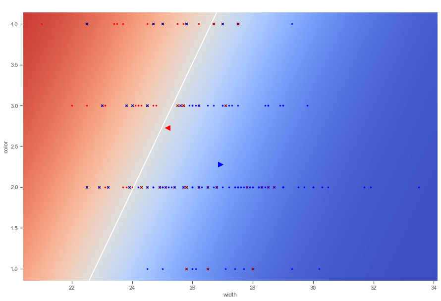
A scatterplot of the explanatory variable values can show the actual y values and use a background color to show the predicted value. This plot shown is derived by the following code:

For a two-class problem, one can show that for LDA
$ \frac{log p_{1}(x)}{1-p_{1}(x)} = log \frac{p_{1}(x)}{p_{2}(x)} = c_{0}+c_{1}x_{1}+..+c_{p}x_{p} $
So it has the same form as logistic regression. The difference is in how the parameters are estimated.
-
Logistic regression uses the conditional likelihood based on P(Y X). - LDA uses the full likelihood based on Pr(X, Y ).
- Despite these differences, in practice the results are often very similar
LDA is useful when n is small, or the classes are well separated, and Gaussian assumptions are reasonable. Also when K > 2.