Lagrangian Methods in Constrained Optimization

An expert is a person who has made all the mistakes that can be made in a very narrow field. - Niles Bohr

In this post, we will examine Lagrange multipliers. We will define them, develop an intuitive grasp of their core principles, and explore how they are applied to optimization problems.

Foundational Concepts

Lagrange multipliers are a mathematical tool employed in constrained optimization of differentiable functions. In the basic, unconstrained scenario, we have a differentiable function $f$ that we aim to maximize (or minimize). We achieve this by locating the extreme points of $f$, where the gradient $\nabla f$ is zero, or equivalently, each partial derivative is zero. Ideally, these identified points will be (local) maxima, but they could also be minima or saddle points. We can distinguish between these cases through various means, including examining the second derivatives or simply inspecting the function values.

let’s look at this simple example where we have $f(x) = 2-x^2$, and we know this function has a maxima at $x=0$, $f(x) = 2$. we can find the maxima by taking the derivative and second derivate of the function to find the maxima of the function.

  • Gradient: $\nabla f =0$.
  • Extreme Point: Solve $\nabla f =0$, which gives x = 0.
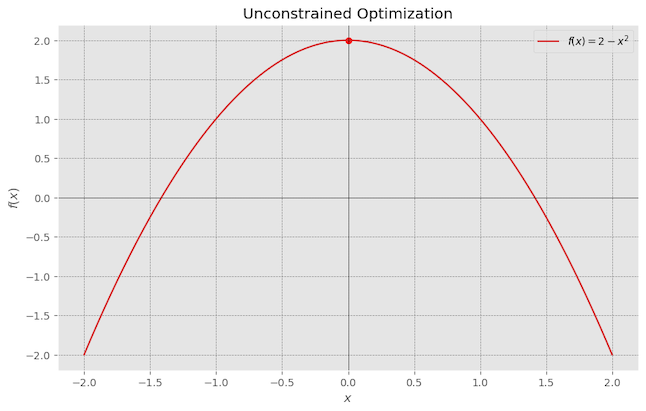
unconstrained

In constrained optimization, we have the same function $f$ to maximize as before. However, we also have restrictions on the points that we’re interested in. The points satisfying our constraints are referred to as the feasible region. A simple constraint on the feasible region is adding boundaries, such as insisting that each $x_{i}$ be positive. Boundaries complicate matters because extreme points on the boundaries generally won’t meet the zero-derivative criterion and must be searched for using other methods.

Building on the previous example, if we add a constraint that, the maximum value of the function $f(x) = 2-x^2$ needs to also meet the constraint that $x=1$. Clearly, the previous maxima value at x=0, where the $f(x)=2$, doesn’t meet that constraint. The maxima for this function $f(x)$, which meets the constraint $g(x)$, is $1$. You can see how finding the function local maxima (minima) using derivative won’t work here because the slope is not zero at this point.

We can use a simple substitution method by substituting the constraint into the main objective function.

  • Objective Function: $f(x) = 2 - x^2$.
  • Contraint: $g(x) = x-1$.

since the constraint is $x=1$, we can substitute this directly into the function:

\[\hspace{5cm} f(1) = 2 - 1^2 = 1\]
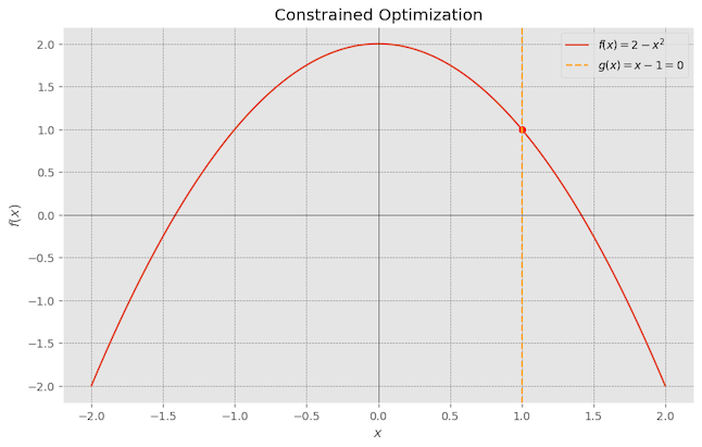
constrained

Now let’s look at a slightly more complex example:

  • Objective function: $f(x,y) = 2 - x^2-2y^2$
  • Constraint: $g(x,y) = x^2-y^2-1=0$

To solve this we can express $y$ in terms of $x$ from the constraint $x^2-y^2=1$:

\[\hspace{5cm} y = \pm \sqrt{1-x^2}\]

Then substitute $y$ back into $f$:

\[\hspace{5cm} f(x,\sqrt{1-x^2}) = 2 - x^2-2(1-x^2) = 2-x^2-2+2x^2 = x^2\] \[\hspace{5cm} f(x,-\sqrt{1-x^2}) = 2 - x^2-2(1-x^2) = 2-x^2-2+2x^2 = x^2\]

The maximum value occurs at $x=\pm1$ and $y=0$. We can see in the below plot that the surface of the function $f(x)$ and the constraint $g(x)$ shown by the red circle on the surface which bounds the maximum value the function $f(x)$ can have. Feel free to play with the figure and observe the function from various points of view to get some intuitive understanding on why the max value occurs at $x=\pm1$ and $y=0$.

Lagrange Multipliers

Intuition

If you recall the gradient of a function points in the direction of steepest ascent. The gradient of the objective function $f$ needs to be perpendicular to the gradient of the constraint function $g$ at the constrained maximum point $x^*$.

  1. The gradient \(\nabla f(x^{*})\) points in the direction of steepest ascent of $f$ at $x^{*}$. If we could move in that direction, we would increase $f$.
  2. The gradient \(\nabla g(x^{*})\) is perpendicular to the constraint surface $g(x)=0$ at constrained maximum $x^*$. Any movement along the constraint surface (i.e., in a direction tangent to the surface) won’t change the value of g.
  3. if \(\nabla f(x^{*})\) was not perpendicular to \(\nabla g(x^{*})\), then it would have a component tangent to a constraint surface. We could move in that allowed direction and increase $f$, contradicting the assumption that $x^*$ is a constrained maximum.
  4. Therefore, for $x^*$ to be a constrained maximum \(\nabla f(x^{*})\) must be perpendicular to the constraint surface. Equivalently \(\nabla f(x^{*})\) must be parallel to \(\nabla g(x^{*})\), i.e. a scalar multiple of it: \(\nabla f(x^*) = \lambda \nabla g(x^{*})\) for some scalar $\lambda$. This is precisely the condition encoded by the Lagrangian.

Here is another function $f(x)$ and a constraint function $g(x)$ shown in red line. You can see that the function $f(x)$ has two maxima’s and minima’s. The gradients of $f(x)$ will point in the direction of those maxima’s. The cosntraint function is a circle, and it’s gradient will point outwards as that is where the constraint function will be maximum.

If we look at the interactive contour plot of the above function $f(x)$ and $g(x)$, where the red arrow is the gradient of $f(x)$, blue arrow is gradient of $g(x)$ and black arrow is vector with the gradients from both functions as components.

As you rotate the blue dot around the circle, you will see where the gradients for both functions become parallel.

<!DOCTYPE html>

ref:Visualizing the Lagrange Multiplier Method

Lagrangian with single constraint

Now going to back our example from substitution method $f(x,y) = 2 - x^2-2y^2$, we will add the constraint using Lagrangian multiplier \(\nabla f(x^*) - \lambda \nabla g(x^{*})\). We will find the gradients of the functions and solving for the critical points gives us potential maxima or minima within the constraint.

\[\hspace{5cm} \mathscr{L}(x,y,\lambda) = f(x,y)-\lambda(x,y)\] \[\hspace{5cm} \mathscr{L}(x,y,\lambda) = 2-x^2-2y^2-\lambda(x^2+y^2-1)\]

Taking the partial derivatives and setting them to zero:

\(\hspace{5cm} \frac{\partial \mathscr{L} }{\partial x} = -2x - 2\lambda x = 0\) This gives us $x=0$ and $\lambda = -1$.

\(\hspace{5cm} \frac{\partial \mathscr{L} }{\partial y} = -4y - 2\lambda y = 0\) This gives us $y=0$ or $\lambda = -2$.

\[\hspace{5cm} \frac{\partial \mathscr{L} }{\partial \lambda} = x^2+y^2 - 1 = 0\]

Case 1: If $x = 0$, then $0^2+y^2=1$. This gives $y=\pm1$. So the points are $(0,1)$ and $(0-1)$.

  • for $(0,1)$, $\lambda=-2$ and $f(0,1)=0$
  • for $(0,-1)$,$\lambda=-2$ and $f(0,-1)=0$

Case 2: if $y=0$, then from the constraints, $x^2+0^2=1$. This gives $x=\pm1$.So the points are $(1,0)$ and $(-1,0)$.

  • for $(1,0)$, $\lambda=-1$ and $f(1,0)=1$
  • for $(-1,0)$, $\lambda=-1$ and $f(-1,0)=1$

We can see the maxima for $f(x,y)$ is $1$ at the points $(1,0)$ and $(-1,0)$.

Constrained Maxima

Lagrangian with Multiple constraints

When optimizing a function $f(x_1, x_2, \ldots, x_n)$ subject to multiple constraints $g_1(x_1, x_2, \ldots, x_n) = 0,g_2(x_1, x_2, \ldots, x_n) = 0 , …, g_m(x_1, x_2, \ldots, x_n) = 0$, the Lagrangian function becomes:

\[\hspace{5cm} \mathscr{L}(x_1, x_2, \ldots, x_n, \lambda_1, \lambda_2, \ldots, \lambda_m) = f(x_1, x_2, \ldots, x_n) - \sum_{i=1}^{m} \lambda_i g_i(x_1, x_2, \ldots, x_n)\]

Each $\lambda_i$ is a Lagrange multiplier associated with the constraint $g_i$ .To find the extrema, we take the partial derivatives of the Lagrangian with respect to each variable and each multiplier, then set them to zero:

\[\hspace{5cm} \frac{\partial \mathscr{L}}{\partial x_j} = 0 \quad \text{for each } j = 1, 2, \ldots, n\] \[\hspace{5cm} \frac{\partial \mathscr{L}}{\partial \lambda_i} = 0 \quad \text{for each } i = 1, 2, \ldots, m\]

This gives us a system of $n + m$ equations.

Lagrangian Encoding

Consider a constrained optimization problem where we want to maximize or minimize an objective function $f(x)$ subject to one or more constraints $g_i(x) = 0$ . The Lagrangian function $\mathscr{L}(x, \lambda)$ is defined as:

\[\hspace{5cm} \mathscr{L}(x, \lambda) = f(x) - \sum_{i} \lambda_i g_i(x)\]

Here:

  • $f(x)$ is the objective function we want to optimize.
  • $g_i(x)$ are the constraint functions.
  • $\lambda_i$ are the Lagrange multipliers associated with each constraint.

The Lagrangian function encapsulates both the objective function and the constraints into a single expression. This allows us to transform the constrained optimization problem into an unconstrained one by finding the saddle points of the Lagrangian.

Think of the Lagrangian as a way to blend the objective function and the constraints. By introducing the multipliers $\lambda_i$ , we penalize deviations from the constraints while still focusing on optimizing $f(x)$.

The multipliers $\lambda_i$ act like balancing weights. They adjust the influence of each constraint on the optimization process. If a constraint is more stringent, the corresponding $\lambda_i$ will be higher, indicating a stronger penalty for violating that constraint. The optimization process using the Lagrangian involves two main steps:

  1. Fix the Multipliers: For a given set of ( $\lambda_i$ ), find the values of ( $x$ ) that maximize (or minimize) ( $\mathscr{L}(x, \lambda)$ ).
  2. Adjust the Multipliers: Adjust the values of ( $\lambda_i$ ) to ensure the constraints ( $g_i(x) = 0$ ) are satisfied.

The Lagrangian helps to formalize the process of finding points where the gradients of the objective function and the constraints are aligned, ensuring the constraints are met while optimizing the objective function.

Duality

Instead of directly solving the original constrained problem (primal problem), we can solve its dual problem. The dual problem focuses on minimizing the Lagrangian with respect to the multipliers, given the values of the primal variables.

For the primal problem: \(\hspace{5cm} \text{maximize } f(x) \text{ subject to } g_i(x) = 0,\)

the dual problem involves:

\[\hspace{5cm} \text{minimizing } \mathscr{L}(x, \lambda) \text{ with respect to } \lambda \text{ subject to the dual constraints}.\]

This transformation often simplifies the problem, especially when the dual problem is easier to solve.

Kuhn-Tucker Theorem

Kuhn-Tucker theorem provides necessary conditions for a solution in nonlinear programming to be optimal, extending the Lagrange multiplier method to handle inequality constraints.

For a problem with both equality and inequality constraints, the Lagrangian is defined as:

\[\hspace{5cm} \mathscr{L}(x, \lambda, \mu) = f(x) - \sum_{i} \lambda_i g_i(x) - \sum_{j} \mu_j h_j(x)\]

Here:

  • $f(x)$ is the objective function.
  • $g_i(x) = 0$ are the equality constraints.
  • $h_j(x) \leq 0$ are the inequality constraints.
  • $\lambda_i$ and $\mu_j$ are the Lagrange multipliers for the equality and inequality constraints, respectively.

Conditions for Optimality

The essential idea behind the KKT conditions is to convert a constrained optimization problem into a system of equations that can be solved to find the optimal solution. The KKT conditions provide necessary conditions for a point to be optimal, meaning that if a point satisfies these conditions, it is a candidate for the optimal solution.

The Kuhn-Tucker conditions are a set of first-order necessary conditions for a solution to be optimal:

Given a nonlinear programming problem:

\[\hspace{5cm} \text{minimize } f(x)\] \[\hspace{5cm} \text{subject to } g_i(x) = 0, \; i = 1, \ldots, m\] \[\hspace{5cm} \text{and } h_j(x) \leq 0, \; j = 1, \ldots, p\]

The Kuhn-Tucker conditions are:

  • Stationarity:
\[\hspace{5cm} \nabla f(x^*) + \sum_{i=1}^m \lambda_i \nabla g_i(x^*) + \sum_{j=1}^p \mu_j \nabla h_j(x^*) = 0\]

The stationarity condition involves setting the gradient of the Lagrangian to zero. This balances the gradient of the objective function $f(x)$ against the weighted gradients of the constraints. The weights are the Lagrange multipliers $\lambda_i$ and $\mu_j$ .

  • Primal Feasibility:
\[\hspace{5cm} g_i(x^*) = 0, \; i = 1, \ldots, m\] \[\hspace{5cm} h_j(x^*) \leq 0, \; j = 1, \ldots, p\]

This condition ensures that the solution \(x^{*}\) satisfies the original equality and inequality constraints. This means \(x^{*}\)
lies within the feasible region defined by these constraints.

  • Dual Feasibility:
\[\hspace{5cm} \mu_j \geq 0, \; j = 1, \ldots, p\]

Dual feasibility requires the Lagrange multipliers associated with the inequality constraints to be non-negative. This is necessary because the multipliers $\mu_j$ represent the shadow prices of the constraints, which must be non-negative to reflect that relaxing a constraint (making it less stringent) would not decrease the objective function.

  • Complementary Slackness:
\[\hspace{5cm} \mu_j h_j(x^*) = 0, \; j = 1, \ldots, p\]

Complementary slackness ensures that for each inequality constraint, either the constraint is active (exactly met) or the corresponding multiplier is zero. If a constraint is not binding (i.e., \(h_j(x^{*}) < 0\) ), its multiplier $\mu_j$ must be zero because the constraint does not affect the solution. Conversely, if the constraint is binding (i.e., \(h_j(x^{*}) = 0\) ), the multiplier $\mu_j$ can be positive, reflecting the cost of tightening the constraint.

Convex Hulls and Optimization

Before we move on to the application aspects, it’s important to mention about the geometrical aspects of the Convex Hulls and it’s relation to the optimization.

Convex Hull

The convex hull of a set of points $S$ in a Euclidean space is the smallest convex set that contains $S$ . It can be visualized as the shape formed by stretching a rubber band around the points. The convex hull of a set $S$ , denoted as $\text{conv}(S)$ , is the set of all convex combinations of points in $S$ :

\[\hspace{5cm} \text{conv}(S) = \left\{ \sum_{i=1}^n \lambda_i x_i \mid x_i \in S, \lambda_i \geq 0, \sum_{i=1}^n \lambda_i = 1 \right\}\]

Convex Hulls and Optimization

When solving optimization problems over a set of points, it is often beneficial to consider the convex hull of these points. If the objective function is linear and the feasible region is defined by the convex hull of a set of points, the optimal solution will lie on the boundary of the convex hull.

Convex Hull

The convex hull contains all feasible solutions to the optimization problem within the smallest convex boundary. The extreme points of the convex hull are the potential candidates for the optimal solution in linear programming problems. The optimal solution for a linear objective function over a convex hull will always be at one of the vertices of the convex hull. By visualizing the direction of the objective function, you can determine which vertex is optimal.

The above plot demonstrates why optimization algorithms like the Simplex Method are effective in linear programming: they move along the edges of the feasible region (convex hull) from vertex to vertex, searching for the optimal solution.

Application of Lagrangian

So we have already seen some introduction of Lagrangian here Balancing MMLU With The Shortest Path Cost Constraints without explicitly calling it as Lagrangian. But lets look at a simple example this time.

Here is a simple graph where we the edges have a cost to traverse and the time it takes. Finding a shortest path from Node $1$ to $6$ is easy and we have looked at those LP formulation. In this case now assume that we have an additional constraint that the total time to traverse from Node $1$ to $6$ should not exceed time $T$.

graph

Lagrangian Relaxation Approach

To tackle the complexity introduced by the transit time constraint, the Lagrangian relaxation method is employed:

Step 1: Penalize Constraint Violation: • Introduce a Lagrangian multiplier ( $\lambda$ ) to penalize violations of the transit time constraint. • Modify the objective function to include this penalty:

\[\hspace{5cm} \mathscr{L}(\lambda) = \min \sum_{(i,j) \in A} (c_{ij} + \lambda t_{ij}) x_{ij} - \lambda T\]

Here,$x_{ij}$ is a binary variable indicating whether arc ( $(i,j)$ ) is included in the path.

Step 2: Relax the Problem: • Remove the complicating constraint ( $\sum_{(i,j) \in A} t_{ij} x_{ij} \leq T$ ) and as we included it in the objective function as a penalty. • The resulting problem is easier to solve since it is now a standard shortest path problem but with modified arc costs.

Effect of Varying ( $\lambda$ )

Case 1: ( $\lambda = 0$ ):

  • The problem reduces to finding the shortest path without considering transit time.
  • The solution is simply the path with the minimum cost.

Case 2: ( $\lambda > 0$ ):

  • As ( $\lambda$ ) increases, the cost of paths with higher transit times increases.
  • The solution path changes, favoring those with lower transit times to avoid high penalties.
  • By adjusting ($\lambda$ ), the algorithm finds paths that balance cost and transit time, providing a trade-off.

Optimization and Bounds

  • The goal is to find the optimal ($\lambda$ ) that maximizes the lower bound on the original problem’s objective value.
  • The optimal value $\mathscr{L}^*$ is found by solving:
\[\hspace{5cm} \mathscr{L}^* = \max \{ \mathscr{L}(\lambda) : \lambda \geq 0 \}\]

Bounding Principle:

  • The obtained lower bound $\mathscr{L}(\lambda)$ is used to gauge the quality of the solution.
  • If $\mathscr{L}(\lambda)$ is close to the actual minimum cost, the solution is considered good.

here is a parametric analysis of the problem. We can see the red line representing cost is minimum with $\lambda=0$, and starts increasing but start plateauing after a while as we increase $\lambda$. The Transit Time line shown the inverse, which also make sense as we increase $\lambda$, we start optimizing for the transit time.

Based on the graph, it appears that we want either $\lambda=3\text{ or }4$, where we meet the latency constraint of 10.

parametric analysis

Restricted Lagrangian Approach

The restricted Lagrangian approach involves iteratively solving a restricted version of the Lagrangian relaxation by only considering a subset of feasible solutions. The key steps are:

  1. Initialize the Set S : Start with a small subset of feasible paths, such as the shortest path without considering the transit time constraint.
  2. Solve the Restricted Lagrangian Problem: Obtain the current lower bound and Lagrange multipliers.
  3. Solve the Lagrangian Subproblem: Find the shortest path considering the modified costs and identify new paths.
  4. Iterate: Expand the set S with new paths until the optimal solution is found.

Assume that now we want to find the optimal solution with maximum Transit time T = 14. The optimal solution is 1->3->2->5->6 based on the restricted Lagrangian approach where $\lambda=4$.

Optimal path: [(1, 3),(3, 2),(2, 5), (5, 6)]
Optimal Lagrange multiplier: 4.0

Here is the code snippet for the relaxed Lagrangian approach.

# Define the graph with given costs and transit times
nodes = [1, 2, 3, 4, 5, 6]
arcs = {
    (1, 2): {'cost': 1, 'time': 10},
    (1, 3): {'cost': 10, 'time': 3},
    (2, 4): {'cost': 1, 'time': 1},
    (2, 5): {'cost': 2, 'time': 3},
    (3, 2): {'cost': 1, 'time': 2},
    (3, 5): {'cost': 12, 'time': 3},
    (3, 4): {'cost': 5, 'time': 7},
    (4, 6): {'cost': 1, 'time': 7},
    (4, 5): {'cost': 10, 'time': 1},
    (5, 6): {'cost': 2, 'time': 2},
}

# Define the maximum allowed transit time
T = 14

# Function to solve the Lagrangian subproblem for a given set of paths and Lagrange multipliers
def lagrangian_subproblem(mu):
    prob = pulp.LpProblem("Lagrangian_Subproblem", pulp.LpMinimize)
    
    # Define decision variables
    x = pulp.LpVariable.dicts("x", arcs, cat='Binary')
    
    # Define the objective function
    prob += pulp.lpSum((arcs[i, j]['cost'] + mu * arcs[i, j]['time']) * x[i, j] for (i, j) in arcs) - mu * T
    
    # Define constraints for flow conservation
    for node in nodes:
        if node == 1:
            prob += pulp.lpSum(x[1, j] for j in nodes if (1, j) in arcs) == 1
        elif node == 6:
            prob += pulp.lpSum(x[i, 6] for i in nodes if (i, 6) in arcs) == 1
        else:
            prob += (pulp.lpSum(x[i, node] for i in nodes if (i, node) in arcs) == 
                     pulp.lpSum(x[node, j] for j in nodes if (node, j) in arcs))
    
    # Solve the problem
    prob.solve()
    
    # Extract the path and transit time
    new_path = [(i, j) for (i, j) in arcs if x[i, j].varValue == 1]
    transit_time = sum(arcs[i, j]['time'] * x[i, j].varValue for (i, j) in arcs)
    
    return new_path, transit_time

# Function to solve the restricted Lagrangian problem
def solve_restricted_lagrangian(S):
    prob = pulp.LpProblem("Restricted_Lagrangian", pulp.LpMaximize)
    
    # Define decision variable
    w = pulp.LpVariable("w")
    mu = {k: pulp.LpVariable(f"mu_{k[0]}_{k[1]}", lowBound=0) for k in arcs}
    
    # Add constraints for each path in S
    for path in S:
        cost_sum = sum(arcs[i, j]['cost'] for (i, j) in path)
        time_sum = sum(arcs[i, j]['time'] for (i, j) in path)
        prob += w <= cost_sum + pulp.lpSum(mu[(i, j)] * arcs[i, j]['time'] for (i, j) in path) - sum(mu[(i, j)] * T for (i, j) in path)
    
    # Define the objective function
    prob += w
    
    # Solve the problem
    prob.solve()
    
    # Extract the Lagrange multipliers and initialize to zero if not set
    mu_values = {k: pulp.value(mu[k]) if pulp.value(mu[k]) is not None else 0 for k in mu}
    return pulp.value(w), mu_values

# Function to solve the constraint generation problem
def constraint_generation():
    # Initialize the set S with the shortest path without considering the transit time constraint
    initial_path = find_path_with_lambda(0)
    S = [initial_path]
    mu = 0
    
    while True:
        # Solve the restricted Lagrangian problem
        lower_bound, mu_values = solve_restricted_lagrangian(S)
        
        # Solve the Lagrangian subproblem with the current mu values
        new_path, transit_time = lagrangian_subproblem(mu)
        
        # Check if the new path violates the transit time constraint
        if transit_time > T:
            # Add the new path to the set S
            if new_path not in S:
                S.append(new_path)
            
            # Update the Lagrange multiplier using subgradient optimization
            subgradient = transit_time - T
            step_size = 1 / (len(S) ** 0.5)
            mu += step_size * subgradient
        else:
            # The current solution is optimal
            optimal_path = new_path
            break
    
    return optimal_path, mu

# Function to find the shortest path for a given lambda value
def find_path_with_lambda(lambda_value):
    prob = pulp.LpProblem("Shortest_Path", pulp.LpMinimize)
    
    # Define decision variables
    x = pulp.LpVariable.dicts("x", arcs, cat='Binary')
    
    # Define the objective function
    prob += pulp.lpSum((arcs[i, j]['cost'] + lambda_value * arcs[i, j]['time']) * x[i, j] for (i, j) in arcs)
    
    # Define constraints for flow conservation
    for node in nodes:
        if node == 1:
            prob += pulp.lpSum(x[1, j] for j in nodes if (1, j) in arcs) == 1
        elif node == 6:
            prob += pulp.lpSum(x[i, 6] for i in nodes if (i, 6) in arcs) == 1
        else:
            prob += (pulp.lpSum(x[i, node] for i in nodes if (i, node) in arcs) == 
                     pulp.lpSum(x[node, j] for j in nodes if (node, j) in arcs))
    
    # Solve the problem
    prob.solve()
    
    # Extract the path
    path = [(i, j) for (i, j) in arcs if x[i, j].varValue == 1]
    return path

# Solve the constraint generation problem
optimal_path, optimal_mu = constraint_generation()

print(f"Optimal path: {optimal_path}")
print(f"Optimal Lagrange multiplier: {optimal_mu}")

References

Written on May 26, 2024