Motivation

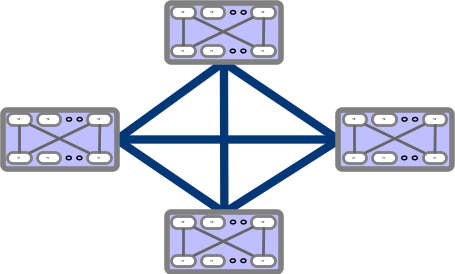
I recently read Google’s latest sigcomm paper: Jupiter Evolving on their Datacenter fabric evolution. It is an excellent paper with tons of good information, and the depth and width show what an engineering thought process should look like. The central theme talks about the challenges faced with deploying and scaling Clos fabrics and how they have evolved by replacing the spine layer with OCS that allows the blocks to be directly connected, calling it Direct connect topology.

If you look closely, the Direct Connect topology resembles Dragonfly+, where you have directly connected blocks.

The paper has many interesting topics, including Traffic and Topology Engineering and Traffic aware routing. One of the most exciting parts to me, which will be understandably missing, is the formulation of Traffic engineering problems as Optimization problems. I would love to see some pseudo-real-world code examples made publicly available.

However, one thing that surprised me the most was from a Traffic characteristics perspective, a Gravity model best described Google’s Inter-Block traffic. When I studied Gravity Model, I thought this was such a simplistic model that I would never see that in real life, but it turns out I was wrong, and it still has practical applicability. This blog will look at the Gravity Model and synthetic traffic generation that follows the gravity model. We will end with an expanded proof given in the appendix section C of Jupiter Evolving.

Introduction

We can divide Traffic Matrix Models into broadly three categories: temporal modelling, spatial Modelling and spatio-temporal modelling.

1. Temporal modelling: In Temporal models, we focus on the time series properties of the traffic matrix.
2. Spatial modelling: In Spatial models, we focus on the properties of traffic between Source and Destination pairs. Gravity Model is an example of that.
3. Spatio-Temporal modelling: As the name suggest, this class of models tries to describe the spatial and temporal structure jointly.

Gravity Model

Gravity modeling is based on Newton’s law of gravitation and has been used in various areas like economy and trade, sociology, retail industry. A few examples are like predicting the movement of people, goods, and services between cities or geographical locations by considering the population and distance factors. In the case of the retail industry, an example is Reilly’s law of retail gravitation.

An application of the Gravity Model for IP Traffic matrix estimation was first proposed by Roughan et al.(4) is based on the total amount of traffic entering and leaving each node in the network and the total traffic in the network. Here, traffic from the source to the destination is modeled as a random process. In its simplest form, it assumes any packet originating from a source to a destination nodes are independent of other packets. Depending on the context, this could be the origin, destination, or ingress and egress nodes. Consequently, the traffic between two nodes is proportional to the total traffic from the source node to the destination node.

In Newton’s law of gravitation, the gravitational force is proportional to the product of the mass of two objects divided by the distance between them squared. Two forces define the general formulation of gravity model: repulsive factor $R_{i}$ associated with “leaving” from $i$ and the attractive force $A_{j}$ associated with going into $j$.$f_{I,j}$ represents the friction factor, which describes the weakening of the forces.

For IP traffic matrix modeling, the friction factors are typically considered constant. This translates to below where $X_{i}^{in}$ is the total traffic entering the network through $i$. $X_{j}^{out}$ is the total traffic exiting the network through $j$ and $X^{total}$ is the total traffic across the network. With that, we get the following for estimating traffic between $i$ and $j$.

The gravity model captures the Spatial structure of the traffic, and the key assumption is the independence between each source $i$ and destination $j$. This gives us $X_{i,j}$ i.e. traffic from $i$ to $j$ as:

or

Where
$X_{i}^{in}$ is the total amount of traffic originating from node i;
$X_{j}^{out}$ is the total amount of traffic destined for node j.

In an ideal network we assume $X^{total} = \sum_{k=1}^{n}X_{k}^{in} = \sum_{k = 1}^{n}X_{k}^{out}$.

There are two important properties of Gravity model:

1. Independence between source and destination traffic holds for any randomly chosen submatrix of the model.
2. Aggregate of the gravity model is also a gravity model.

Synthetic Generation

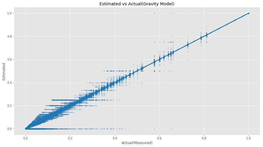
We can use synthetic traffic if we need access to real-world traffic. Below is a sample of synthetic traffic matrix generation conforming to the Gravity model. There are multiple ways to generate synthetic traffic, from independent exponential random variables to more complicated ways using sampling algorithms like MCMC (Markov Chain Monte Carlo). Below is an example of Synthetic traffic that follows the Gravity model using exponential random variables. The sample code is available in the Appendix.

Expanded appendix Proof

In appendix section C of Jupiter Evolving, a lemma is presented with proof, i.e., if a network can support a gravity-model traffic matrix where aggregate egress and ingress traffic demands are the same, then the network can support the demand after the aggregate demand at one node decreases. So this means that given that aggregate demands are the same, a reduction of demand at a node $v$ will lead to an increase in demand from node $i$ to other nodes excluding $v$. Still, that increase in demand can be re-routed via $v$ because reduction at $v$ frees up sufficient capacity.

While going through the proof, I had to reach out to the Jupiter Evolving team for some clarity, and I am writing the expanded proof below in case someone else finds it useful.

Proof

Assuming Gravity model, the traffic demand from $i$ to $j$ is given by $D_{ij} = \frac{D_{i}D_{j}}{\sum_{k\in V}D_{k}}$. If the aggregate demand at $u$ decreases from $D_{u}$ to $D’_{u}$, the demand From $i$ to $u$ reduces by:

In simple words, it’s saying $c_{iv} = OriginalTrafficDemand - ReducedTrafficDemand$. The demand from $i$ to $j$ increases by:

if $c_{iv} \gt \sum_{j\in V\setminus{i,v}}b_{ij}$, then the increased demand from $i$ to all other nodes except $v$ can transit through $v$ as it frees sufficient capacity. In order to hold this true, $c_{iv} - \sum_{j\in V\setminus{i,v}}b_{ij} \gt 0$ needs to hold true. Below is the proof for that.

$\sum_{k\in V}D_{k} - \sum_{j\in V\setminus{i,v}}D_{j}$ is the sum over all nodes in $V$ minus the sum over all nodes in $V$ except $i$ and $v$. This is equivalent to $D_{i}+D_{v}$. Substituting $\sum_{k \in V}D_{k}- \sum_{j\in V\setminus{i,v}}D_{j} = D_{i}+D_{v}$

substituting $\sum_{k \in V}D_{k}- \sum_{j\in V\setminus{i,v}}D_{j} = D_{i}+D_{v}$

We know that demand at $v$ reduced from \(D_{v} \hspace{1mm} to \hspace{1mm} D'_{v}\), so \(D_{v}-D'_{v} \ge 0\). Rest of the terms are also positive. So we proved that $c_{iv} \ge b_{ij}$.

Conclusion

We presented model classification into three categories: purely temporal, purely spatial, and spatio-temporal models. The gravity model is a spatial model, and we presented a brief intro to the Gravity model and how it applies to the IP traffic matrix. The gravity model usefulness comes from its simplicity, and google’s latest sigcom paper suggests that their inter-block traffic follows the Gravity model, so there is undoubtedly a real-life example of the Gravity model. We looked at a sample code for generating Gravity model traffic and then an expanded proof for the Gravity model.

Appendix

import numpy as np
import pandas as pd
import scipy.stats as st

def rmse(predictions, targets):
    return np.sqrt(((predictions - targets) ** 2).mean())

def get_traffic_matrix(n, scale: float = 100, fixed_total: float = None) -> np.ndarray:
    """
    Creates a traffic matrix of size n x n using the gravity model with independent exponential distributed weight vectors
    :n: size of network (# communication nodes)
    :scale: used for generating the exponential weight vectors
    :fixed_total: if not None, the sum of all demands are scaled to this value
    :returns: n x n traffic matrix as numpy.ndarray
    """
    t_in = np.array([st.expon.rvs(size=n, scale=scale)])
    t_out = np.array([st.expon.rvs(size=n, scale=scale)])

    t = (np.sum(t_in) + np.sum(t_out)) / 2  # assumption that sum(t_in) == sum(t_out) == t

    # probability matrix
    p_in = t_in / np.sum(t_in)
    p_out = t_out / np.sum(t_out)
    p_matrix = np.matmul(p_in.T, p_out)

    # traffic matrix
    t_matrix = p_matrix * t

    if fixed_total:
        multiplier = fixed_total / np.sum(t_matrix)
        t_matrix *= multiplier

    return t_matrix

## Get a Gravity Model Traffic Matrix for 500 Nodes with Total traffic limited to 1000000 and Create a DataFrame.
traffic_matrix2 = get_traffic_matrix(n=500, fixed_total=1000000)
df_tm_max = pd.DataFrame(traffic_matrix2)
## Total In and Total Out
total_in=  df_tm_max.sum(axis=1)
total_out = df_tm_max.sum(axis=0)
## Total= Total Out = Total In. Picking Total Out
total = df_tm_max.sum(axis=0).sum()

## Create a Traffic Matrix dataframe of 500 as Src/Dst Nodes and fill with one.
df_tm_gv = pd.DataFrame(1, index=total_in.index, columns=total_out.index)
## Resulting Gravity Matrix = (Total_in * Total_Out)/Total
results = ((df_tm_gv.multiply(total_in, axis='index') * total_out)/total).round(1)

## Normalize the resulting matrix.
results_norm = (results - results.min())/(results.max() - results.min())
## Normalize the synthetic Traffic Matrix 
df_tm_max_norm = (df_tm_max-df_tm_max.min())/(df_tm_max.max() - df_tm_max.min())

## Plot the Estimated vs Generated Traffic Matrix.
plt.scatter(df_tm_max_norm.values, results_norm.values, alpha=0.1, color="tab:blue", marker=".")
_= plt.plot(df_tm_max_norm.values, df_tm_max_norm.values, color="tab:blue",linestyle="--")

References

1. Jupiter Evolving
2. Internet Traffic Matrics: A Primer
3. Dragonfly+: Low Cost Topology for Scaling Datacenters
4. Experience in Measuring Backbone Traffic Variability: Models, Metrics, Measurements and Meaning