Generalized Linear Models(GLMs) Rough Notes
In case of Linear Models, we assume a linear relationship between the mean of the response variable and a set of explanatory variables with inference assuming that response variable has a Normal conditional distribution with constant variance. The Generalized Linear Model permits the distribution for the Response Variable other than the normal and permits modeling of non-linear functions of the mean. Linear models are special case of GLM.
GLM extends normal linear models to encompass non-normal distributions and equating linear predictors to nonlinear functions of the mean. The fundamental premise is that
1) We have a linear predictor. $\eta_{i} = a + Bx$.
2) Predictor is linked to the fitted response variable value of $Y_{i}, \mu_{i}$
3) The linking is done by the link function, such that $g(\mu_{i}) = \eta_{i} $. For example, for a linear function $\mu_{i} = \eta_{i}$, for an exponential function, $log(\mu_{i}) = \eta_{i}$
$ g(\mu_{i}) = \beta_{0} + \beta_{1}x_{i1} + … + \beta_{p}x_{ip} $
The link function $g(\mu_{i})$ is called the link function.
Some common examples:
- Identity: $\mu = \eta$, example: $\mu = a + bx$
- Log: $log(\mu) = \eta$, example: $\mu = e^{a + bx}$
- Logit: $logit(\mu) = \eta$, example: $\mu = \frac{e^{a + bx}}{1+ e^{a + bx}}$
- Inverse: $\frac{1}{\mu} = \eta$, example: $ \mu = (a+bx)^{-1}$
GLMs for Normal, Binomial, and Poisson Responses
For continuous response variables, the most important GLMs are normal linear models. Models assume independent response observations $Y_{i} \sim N(\mu_{i}, \sigma^2)$ for i = 1,…, n, and use the identity link function for which $ \mu_{i} = \beta_{0} + \beta_{1}x_{i1} + … + \beta_{p}x_{ip}$.
Other distributions like Gamma distribution is useful when response variables are non-negative and variability increases with mean.
For Categorical response variables, we model the outcome in a particular category. When the response variable is
binary, representing Success and Failure outcomes by 1 and 0, observation i has probabilities
$P(Y_{i} = 1) = \pi_{i}$ and $P(Y_{i} = 0) = 1-\pi_{i}$. The probability $\pi_{i}$ is not compatible with linear predictor
$\beta_{0} + \beta_{1}x_{i1} + … + \beta_{p}x_{ip}$ because it falls between 0 and 1 whereas the linear predictor can
take any real number value. we can use a link function to transform probabilities so that they can take any real number
values using canonical link function for $\mu_{i} = \pi_{i}$ is $log[\frac{\mu_{i}}{1-\mu_{i}}]$, called as logit.
Like linear predictor, logit can take any real number value. GLMs using the logit link function have the form
$ log(\frac{\mu_{i}}{1-\mu_{i}}) = \beta_{0} + \beta_{1}x_{i1} + … + \beta_{p}x_{ip}, \ i = 1,…,n. $
This is called logistic regression models.
When the response variable has counts for the outcomes, the simples probability distribution for response variable is Poisson. The log function is then the most common link function. The mean of a count response must be non-negative and its log can take any real number value, like a linear predictor. A GLM using the log function is called a loglinear model.
$ log \ \mu_{i} = \beta_{0} + \beta_{1}x_{i1} + … + \beta_{p}x_{ip}, \ i = 1,…,n. $
With the assumption that response variable has a Poisson distribution, it is called a Poisson log-linear model. The negative binomial log-linear model permits overdispersion where count data in which the variance exceeds the mean. Remember in case of Poisson we have only one variable mean, and we expect the variance=mean.
Below is the Scottish Hill Runners Race data(https://scottishhillrunners.uk/) with Distance and Climb being explanatory variable and record times being the response variable for Men and Women.
## Example
## Here is the data of Scottish HIll Runners Assosciations a list of hill races in Scotland.
Races = pd.read_csv('data/ScotsRaces.dat', sep='\s+')
Races2 = Races.drop(['timeM'], axis=1) # Dropping Male Times
## Applying OLS
fitdc = smf.ols(formula="timeW ~ distance + climb", data=Races2).fit()
print(fitdc.summary())

                            OLS Regression Results
==============================================================================
Dep. Variable:                  timeW   R-squared:                       0.964
Model:                            OLS   Adj. R-squared:                  0.963
Method:                 Least Squares   F-statistic:                     872.6
Date:                Sun, 30 Oct 2022   Prob (F-statistic):           1.10e-47
Time:                        15:48:16   Log-Likelihood:                -274.24
No. Observations:                  68   AIC:                             554.5
Df Residuals:                      65   BIC:                             561.1
Df Model:                           2
Covariance Type:            nonrobust
==============================================================================
                 coef    std err          t      P>|t|      [0.025      0.975]
------------------------------------------------------------------------------
Intercept    -14.5997      3.468     -4.210      0.000     -21.526      -7.674
distance       5.0362      0.168     29.919      0.000       4.700       5.372
climb         35.5610      3.700      9.610      0.000      28.171      42.951
==============================================================================
Omnibus:                        1.739   Durbin-Watson:                   1.805
Prob(Omnibus):                  0.419   Jarque-Bera (JB):                1.043
Skew:                          -0.158   Prob(JB):                        0.594
Kurtosis:                       3.518   Cond. No.                         53.5
==============================================================================

Notes:
[1] Standard Errors assume that the covariance matrix of the errors is correctly specified.
## Applying GLM. Default identity link function is Gaussian.
fitdc.glm = smf.glm(formula="timeW ~ distance + climb", data=Races2).fit()
print(fitdc.glm.summary())
                 Generalized Linear Model Regression Results
==============================================================================
Dep. Variable:                  timeW   No. Observations:                   68
Model:                            GLM   Df Residuals:                       65
Model Family:                Gaussian   Df Model:                            2
Link Function:               identity   Scale:                          195.00
Method:                          IRLS   Log-Likelihood:                -274.24
Date:                Sun, 30 Oct 2022   Deviance:                       12675.
Time:                        15:48:16   Pearson chi2:                 1.27e+04
No. Iterations:                     3
Covariance Type:            nonrobust
==============================================================================
                 coef    std err          z      P>|z|      [0.025      0.975]
------------------------------------------------------------------------------
Intercept    -14.5997      3.468     -4.210      0.000     -21.397      -7.802
distance       5.0362      0.168     29.919      0.000       4.706       5.366
climb         35.5610      3.700      9.610      0.000      28.309      42.813
==============================================================================
The model fit $\hat\mu$ = -14.6 + 5.04(distance) + 35.56(climb) indicates that adjusted for climb the predicted record time increases by 5.04mins for every additional km of distance. adjusted for distance, the predicted record time increases by 35.56mins for every additional km of climb.
The parameter estimates are identical to OLS, but inference about individual coefficients differs slightly because the glm function uses normal distributions for the sampling distributions (regardless of the assumed distribution for Y ), whereas the ols function uses the t distribution, which applies only with normal responses.
An example for House selling prices.
## Example
## Model House Selling Prices
Houses = pd.read_csv('data/Houses.dat', sep='\s+')
Houses['house'] = Houses['new'].apply(lambda x: 'old' if x==0 else 'new')
print(Houses.head(5))
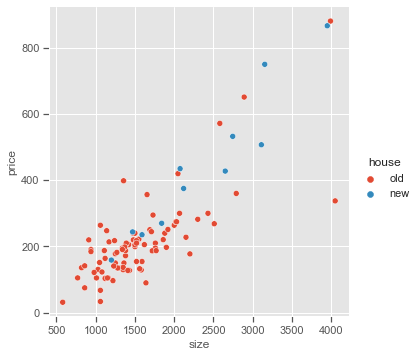
_= sns.pairplot(x_vars=['size'], y_vars=['price'], data=Houses, hue='house', height=5)
   case   price  size  new  taxes  bedrooms  baths house
0     1  419.85  2048    0   3104         4      2   old
1     2  219.75   912    0   1173         2      1   old
2     3  356.55  1654    0   3076         4      2   old
3     4  300.00  2068    0   1608         3      2   old
4     5  239.85  1477    0   1454         3      3   old
fit1 = smf.glm(formula = 'price ~ size + new + size:new', data = Houses,family = sm.families.Gaussian()).fit()
print(fit1.summary())

                 Generalized Linear Model Regression Results
==============================================================================
Dep. Variable:                  price   No. Observations:                  100
Model:                            GLM   Df Residuals:                       96
Model Family:                Gaussian   Df Model:                            3
Link Function:               identity   Scale:                          6083.6
Method:                          IRLS   Log-Likelihood:                -575.52
Date:                Sun, 30 Oct 2022   Deviance:                   5.8402e+05
Time:                        15:48:17   Pearson chi2:                 5.84e+05
No. Iterations:                     3
Covariance Type:            nonrobust
==============================================================================
                 coef    std err          z      P>|z|      [0.025      0.975]
------------------------------------------------------------------------------
Intercept    -33.3417     23.282     -1.432      0.152     -78.973      12.290
size           0.1567      0.014     11.082      0.000       0.129       0.184
new         -117.7913     76.511     -1.540      0.124    -267.751      32.168
size:new       0.0929      0.033      2.855      0.004       0.029       0.157
==============================================================================
The interaction term between House Size and New is highly significant. From the size effect and the interaction term, the estimated effect on selling price of a square foot increase in size 0.157 for older homes and 0.157 + 0.093 = 0.250 for newer homes.
However, the scatter plot shows that the variability in prices could be greater for higher house sizes which breaks the OLS assumption of constant variability in response variable. Using Gamma distribution, the deviation $\sigma = \frac{\mu}{\sqrt{k}}$ for the shape parameter k.
gamma_mod = smf.glm(formula = 'price ~ size + new + size:new', data = Houses,
                    family = sm.families.Gamma(link = sm.families.links.identity)).fit()
print(gamma_mod.summary())
                 Generalized Linear Model Regression Results
==============================================================================
Dep. Variable:                  price   No. Observations:                  100
Model:                            GLM   Df Residuals:                       96
Model Family:                   Gamma   Df Model:                            3
Link Function:               identity   Scale:                         0.11020
Method:                          IRLS   Log-Likelihood:                -559.60
Date:                Sun, 30 Oct 2022   Deviance:                       10.563
Time:                        15:48:17   Pearson chi2:                     10.6
No. Iterations:                    11
Covariance Type:            nonrobust
==============================================================================
                 coef    std err          z      P>|z|      [0.025      0.975]
------------------------------------------------------------------------------
Intercept    -11.1764     19.461     -0.574      0.566     -49.320      26.967
size           0.1417      0.015      9.396      0.000       0.112       0.171
new         -116.8569     96.873     -1.206      0.228    -306.725      73.011
size:new       0.0974      0.055      1.769      0.077      -0.011       0.205
==============================================================================
As we can see that interaction term is not significant anymore while using Gamma distribution, reflecting the greater variability in the response as the mean increases for that GLM.
From the size effect, the estimated effect on selling price of a square foot increase in size 0.142 for older homes. The dispersion parameter estimate is $\frac{1}{\hat{k}}$ = 0.1102. The estimated standard deviation $\hat\sigma$ of the conditional distribution of $Y$ relates to the estimated mean selling price $\hat\mu$ by $\hat\sigma= \frac{\hat\mu}{\sqrt{\hat{k}}} = \sqrt{0.1102}\hat\mu = 0.332\hat\mu$.
For example, when the estimated mean selling price $ $100,000$, $\hat\sigma = $33,200$, when it is $ $500,000$ then $\hat\sigma = $166,000$
The Deviance
Deviance is a goodness-of-fit statistic. It is a generalization of the idea of using the sum of squares of residuals(SSR) in ordinary least squares to cases where model-fitting is achieved by maximum likelihood.
A Saturated Model is the model that perfectly fits the data. In this case, the number of parameters is equal to the number of data points. This is considered to be the perfect model as it takes into account all the variance in the data and has the maximum achievable likelihood.
A Null Model is the opposite with only one parameter, which is the intercept. This is essentially the mean of all the data points.
The Proposed Model is considered the best fit and has a number of parameters in-between the Null and Saturated Models. This is what we are trying to fit.
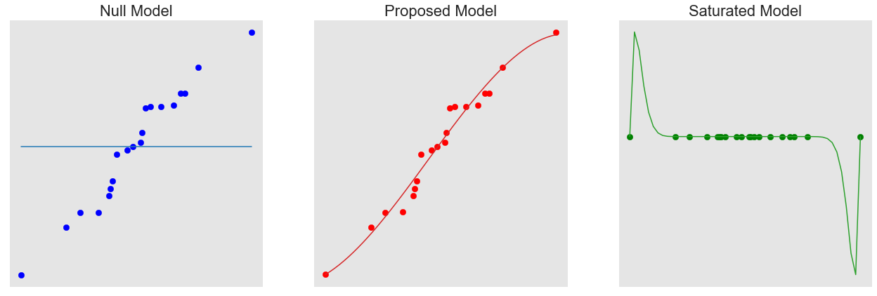
We observe that the Null Model is not good at categorising the data, however on the other hand, the Saturated Model is over-fitting. Proposed Model it generalising the data the best.
Deviance is defined as the difference between the Saturated and Proposed Models and can be thought as how much variation in the data does our Proposed Model account for. Therefore, the lower the deviance, the better the model.
$ D(y;\hat\mu) = 2 log[\frac{max. \ likelihood \ for \ saturated \ model}{\ max. \ likelihood \ for \ proposed \ model}] \ = 2[L(y;y) - L(\hat\mu;y)] $
For Normal Distribution Log-Likelihood for our proposed model
$ L(\hat\mu;y) = \log[\prod_{i=1}^{n}(\frac{1}{\sqrt{2\pi}\sigma}e^{-(y_{i}-\mu_{i})^2/2\sigma^2})] = -n\log(\sqrt{2\pi}\sigma)-\frac{\sum_{i=1}^{n}(y_{i}-\mu_{i})^2}{2\sigma^2} $
for Saturated model, the first term in $L(y;y)$ is the same as in $L(\hat\mu;y)$ but the second term equals 0, because $\hat\mu_{i} = y_{i}$. Therefore
$ D(y;\hat\mu) = 2[L(y;y) - L(\hat\mu;y)] = (\frac{1}{\sigma^2})\sum_{i=1}^{n}(y_{i} - \hat\mu_{i})^2 $
In practice, $\sigma^2$ is unknown.
Example with Covid-19 Data
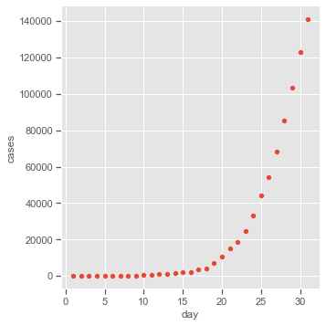
Covid-19 cases in the US in march 2020. Covid-19 data set using normal and gamma GLMs. We fit:
1) normal linear model for the log counts (i.e., assuming a lognormal distribution for the response)
2) GLM using the log link for a normal response
3) GLM using the log link for a gamma response.
Covid = pd.read_csv('data/Covid19.dat', sep='\s+')
sns.pairplot(x_vars=['day'], y_vars=['cases'], data=Covid,  height=5)
fit1 = smf.ols(formula='np.log(cases) ~ day', data=Covid).fit()
print(fit1.summary())
                            OLS Regression Results
==============================================================================
Dep. Variable:          np.log(cases)   R-squared:                       0.994
Model:                            OLS   Adj. R-squared:                  0.993
Method:                 Least Squares   F-statistic:                     4540.
Date:                Sun, 30 Oct 2022   Prob (F-statistic):           2.02e-33
Time:                        15:48:18   Log-Likelihood:                 2.8442
No. Observations:                  31   AIC:                            -1.688
Df Residuals:                      29   BIC:                             1.180
Df Model:                           1
Covariance Type:            nonrobust
==============================================================================
                 coef    std err          t      P>|t|      [0.025      0.975]
------------------------------------------------------------------------------
Intercept      2.8439      0.084     33.850      0.000       2.672       3.016
day            0.3088      0.005     67.377      0.000       0.299       0.318
==============================================================================
Omnibus:                        3.668   Durbin-Watson:                   0.273
Prob(Omnibus):                  0.160   Jarque-Bera (JB):                3.123
Skew:                          -0.770   Prob(JB):                        0.210
Kurtosis:                       2.785   Cond. No.                         37.7
==============================================================================

Notes:
[1] Standard Errors assume that the covariance matrix of the errors is correctly specified.
fit2 = smf.glm(formula = 'cases ~ day', family =
               sm.families.Gaussian(link = sm.families.links.log), data = Covid).fit()
print(fit2.summary())
                 Generalized Linear Model Regression Results
==============================================================================
Dep. Variable:                  cases   No. Observations:                   31
Model:                            GLM   Df Residuals:                       29
Model Family:                Gaussian   Df Model:                            1
Link Function:                    log   Scale:                      1.1565e+07
Method:                          IRLS   Log-Likelihood:                -295.07
Date:                Sun, 30 Oct 2022   Deviance:                   3.3540e+08
Time:                        15:48:19   Pearson chi2:                 3.35e+08
No. Iterations:                     9
Covariance Type:            nonrobust
==============================================================================
                 coef    std err          z      P>|z|      [0.025      0.975]
------------------------------------------------------------------------------
Intercept      5.3159      0.168     31.703      0.000       4.987       5.645
day            0.2129      0.006     37.090      0.000       0.202       0.224
==============================================================================
fit3 = smf.glm(formula='cases ~ day', family =
               sm.families.Gamma(link = sm.families.links.log), data = Covid).fit()
print(fit3.summary())
                 Generalized Linear Model Regression Results
==============================================================================
Dep. Variable:                  cases   No. Observations:                   31
Model:                            GLM   Df Residuals:                       29
Model Family:                   Gamma   Df Model:                            1
Link Function:                    log   Scale:                        0.044082
Method:                          IRLS   Log-Likelihood:                -237.69
Date:                Sun, 30 Oct 2022   Deviance:                       1.4239
Time:                        15:48:19   Pearson chi2:                     1.28
No. Iterations:                    18
Covariance Type:            nonrobust
==============================================================================
                 coef    std err          z      P>|z|      [0.025      0.975]
------------------------------------------------------------------------------
Intercept      2.8572      0.077     36.972      0.000       2.706       3.009
day            0.3094      0.004     73.388      0.000       0.301       0.318
==============================================================================
All three models assume an exponential relationship for the response over time, but results are similar with models (1) and (3) because they both permit the variability of the response to grow with its mean.
The gamma GLM has fit $\log(\hat\sigma) = 2.857 + 0.309x_{i}$. We can obtain the estimated mean by exponentiation both sides yielding $(\hat\sigma) = \exp(2.857 + 0.309x_{i}) = 17.41(1.36)^{x_{i}}$. When we use log link function, model affects are multiplicative. The estimated mean on day x+1 = mean on x multiplied by 1.36, i.e. the mean increases by 36%.
Logistic Regression for Binary Data
GLMs for binary response assume a binomial distribution for the response variable. The most common link function for binomial GLMs is the logit.
For binary data, each observation $y_{i}$ takes value 0 or 1. Then, $\mu_{i} = E(Y_{i}) = P(Y_{i})$,
denoted by $\pi_{i}$. Let logit($\pi_{i}$) denote $\log[\pi_{i}/(1-\pi_{i})]$. The logistic regression model
with p explanatory variables is
$ logit(\pi_{i}) = \log(\frac{\pi_{i}}{1-\pi_{i}}) = \beta_{0}+\beta_{1}x_{i1}+…+\beta_{p}x_{ip} $
With some basic algebra manipulation, we can say
$ P(Y_{i}=1) = \pi_{i} = \frac{\ \exp(\beta_{0}+\beta_{1}x_{i1}+…+\beta_{p}x_{ip})}{1+\ exp(\beta_{0}+\beta_{1}x_{i1}+…+\beta_{p}x_{ip})} $
Parameter Interpretation
For a single explanatory variable
$ P(Y=1) = \frac{\ \exp(\beta_{0}+\beta_{1}x)}{1+\ exp(\beta_{0}+\beta_{1}x)} \ and \ P(Y=0) = 1-P(Y=1)= \frac{1}{1+\ exp(\beta_{0}+\beta_{1}x)} $
the curve for P(Y=1) is monotone in x: when $\beta_{1} > 0, P(Y=1)$ increases as x increases. When $\beta_{1} < 0, P(Y=1)$
decreases as x increases.When $\beta_{1}=0$, the logistic curve flattens to a horizontal line. As x changes, P(Y=1)
approaches 1 at the same rate that it approaches 0. The model has P(Y=1) = 0.50 when logit(P(Y=1)) = log(.50/.50) = log(1) = 0 = $\beta_{0}+\beta_{1}x$ which occurs at $x = \frac{-\beta_{0}}{\beta_{1}}$.
With multiple explanatory variables, P(Y=1) is monotone in each explanatory variable according to the sign of its coefficients.
We can also interpret the magnitude of $\beta_{1}$. A straight line drawn tangent to the curve at any particular value describes the rate of the change in P(Y=1) at that point. Using the logistic regression formula for P(Y=1), the slope is
$ \frac{\partial P(Y=1)}{\partial x} = \frac{\partial }{\partial x}[\frac{\ exp(\beta_{0}+\beta_{1}x)}{ 1+ \ exp(\beta_{0}+\beta_{1}x)}] = \beta_{1}\frac{\ exp(\beta_{0}+\beta_{1}x)}{[1+ \ exp(\beta_{0}+\beta_{1}x)]^2}= \beta_{1}P(Y=1)[1-P(Y=1)] $
The slope is steepest, and equals $\beta_{1}/4$ when P(Y=1) = 1/2. The slop decreases towards 0 as P(Y=1) moves towards 0 or 1.
An alternate interpretation for $\beta_{1}$ uses the odds of success,
$ odds = \frac{P(Y=1)}{P(Y=0)} $
The odds can take any non-negative value. With an odds of 3, we expect 3 success for every failure. with an odds of 1/3, we expect 1 success for every 3 failures. The log of the odds is the logit. From the logistic regression formulas for P(Y=1) and P(Y=0), the odds with this model are
$ \frac{P(Y=1)}{P(Y=0)} = \frac{e^{\beta_{0}+\beta_{1}x}/(1+e^{\beta_{0}+\beta_{1}x})}{1/{ (1+ e^{\beta_{0}+\beta_{1}x}})} = = e^{(\beta_{0}+\beta_{1}x)} = e^{\beta_{0}}(e^{\beta_{1}})^x $
The odds have exponential relationship with $x$. A 1-unit increase in $x$ has a multiplicative impact of $\exp^{\beta_{1}}$. The odds at x = u+1 equals the odds at x = u multiplied by $\exp^{\beta_{1}}$. Equivalently, $\exp^{\beta_{1}}$ is the ratio of the odds at x+1 divided by the odds at x, which is called an odds ratio.
For a logistics regression model with multiple explanatory variables, the odds are
$ \frac{P(Y=1)}{P(Y=0)} = \exp^{\beta_{0}}(\exp^{\beta_{1}})^{x_{1}}…(\exp^{\beta_{j}})^{x_{j}}…(\exp^{\beta_{p}})^{x_{p}} $
Example
Let’s model the probability of death for flour beetles after five hours of exposure to various log-dosages of gaseous carbon disulfide (in mg/liter). The response variable is binary with y = 1 for death and y = 0 for survival.
Beetles = pd.read_csv('data/Beetles_ungrouped.dat',sep='\s+')
Beetles.head(5)

       x	y
0	1.691	1
1	1.691	1
2	1.691	1
3	1.691	1
4	1.691	1
fit = smf.glm('y ~ x', family = sm.families.Binomial(), data=Beetles).fit()
print(fit.summary())
                 Generalized Linear Model Regression Results
==============================================================================
Dep. Variable:                      y   No. Observations:                  481
Model:                            GLM   Df Residuals:                      479
Model Family:                Binomial   Df Model:                            1
Link Function:                  logit   Scale:                          1.0000
Method:                          IRLS   Log-Likelihood:                -186.18
Date:                Sun, 30 Oct 2022   Deviance:                       372.35
Time:                        15:48:20   Pearson chi2:                     436.
No. Iterations:                     6
Covariance Type:            nonrobust
==============================================================================
                 coef    std err          z      P>|z|      [0.025      0.975]
------------------------------------------------------------------------------
Intercept    -60.7401      5.182    -11.722      0.000     -70.896     -50.584
x             34.2859      2.913     11.769      0.000      28.576      39.996
==============================================================================
logdose = Beetles.x.unique() ## Unique x values
yx = pd.crosstab(Beetles['y'],Beetles['x'], normalize= 'columns') ## Get the proportions of death/survival.
y_prop=yx.iloc[1]
## Func returning the P(Y=1) with coefficient values derived from the fit
def f(t):
    return np.exp(fit.params[0] + fit.params[1]*t)/(1 + np.exp(fit.params[0] + fit.params[1]*t))
t1 = np.arange(1.65, 1.95, 0.0001)
fig, ax = plt.subplots(figsize=(8,5))
plt.plot(t1, f(t1),'tab:blue')
plt.scatter(logdose, y_prop, s=10, color='tab:red')
ax.set(xlabel='x', ylabel='P(Y=1)')
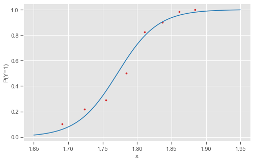
As $x$ increases from lowest to highest dosage, P(Y=1) increases with value .50 at $x = -\beta_{0}/\beta_{1} = 60.74/34.29 = 1.77$. The effect is substantial. The log-dosage has a range of only 1.884 - 1.691 = 0.19, so it not sensible to consider the effect for a 1-unit change in x. For each 0.01 increase in the log dosage, the estimated odds of death multiply by $(\exp^{0.01})^{34.286}$ = 1.41.
The 95% wald confidence interval for $0.01\beta$ is $0.01[34.286\pm1.96(2.913)]$ which is $(2.86, 0.400)$.
To predict the probability of death for new values of x (dosage), 1.7 and 1.8 is given by
x_new = pd.DataFrame({'x': [1.7,1.8]})
y_pred = fit.predict(x_new); print(y_pred)
0    0.079143
1    0.726023
dtype: float64
## Repeating for Grouped Data
Beetles2=pd.read_csv('data/Beetles.dat',sep='\s+')
Beetles2.head(5)
	logdose	live	dead	n
0	1.691	53	6	59
1	1.724	47	13	60
2	1.755	44	18	62
3	1.784	28	28	56
4	1.811	11	52	63
fit = smf.glm('dead + live ~ logdose', data = Beetles2,family = sm.families.Binomial()).fit()
print(fit.summary())
                 Generalized Linear Model Regression Results
==============================================================================
Dep. Variable:       ['dead', 'live']   No. Observations:                    8
Model:                            GLM   Df Residuals:                        6
Model Family:                Binomial   Df Model:                            1
Link Function:                  logit   Scale:                          1.0000
Method:                          IRLS   Log-Likelihood:                -18.657
Date:                Sun, 30 Oct 2022   Deviance:                       11.116
Time:                        15:48:21   Pearson chi2:                     9.91
No. Iterations:                     6
Covariance Type:            nonrobust
==============================================================================
                 coef    std err          z      P>|z|      [0.025      0.975]
------------------------------------------------------------------------------
Intercept    -60.7401      5.182    -11.722      0.000     -70.896     -50.584
logdose       34.2859      2.913     11.769      0.000      28.576      39.996
==============================================================================
The deviance differs, since now the data file has 8 observations instead of 481, but the estimates and standard errors are identical.
Poisson LogLinear Models for Count Data
For modelling response variables which are counts, use Poisson log-linear models. Examples: How many times a person has
been arrested. Remember that for Poisson distribution, it is only defined by a single parameter and because of that mean=variance.
LogLinear Model is
$ log \mu_{i} = \beta_{0} + \beta_{1}x_{i1}+…+\beta_{p}x_{ip}, i = 1,…,n. $
The Poisson LogLinear Model assumes that the counts are independent Poisson Random variables. Log is the canonical link function for the Poisson.
Example
Poisson log-linear models for data on female horseshoe crabs, in which the response variable is the number of male satellites during a mating season.
Crabs = pd.read_csv('data/Crabs.dat', sep='\s+')
print(Crabs.head())
fit = smf.glm('sat ~ weight + C(color)', family=sm.families.Poisson(), data=Crabs).fit() # Default is log link.
print(fit.summary())
   crab  sat  y  weight  width  color  spine
0     1    8  1    3.05   28.3      2      3
1     2    0  0    1.55   22.5      3      3
2     3    9  1    2.30   26.0      1      1
3     4    0  0    2.10   24.8      3      3
4     5    4  1    2.60   26.0      3      3

                 Generalized Linear Model Regression Results
==============================================================================
Dep. Variable:                    sat   No. Observations:                  173
Model:                            GLM   Df Residuals:                      168
Model Family:                 Poisson   Df Model:                            4
Link Function:                    log   Scale:                          1.0000
Method:                          IRLS   Log-Likelihood:                -453.55
Date:                Sun, 30 Oct 2022   Deviance:                       551.80
Time:                        15:48:21   Pearson chi2:                     535.
No. Iterations:                     5
Covariance Type:            nonrobust
=================================================================================
                    coef    std err          z      P>|z|      [0.025      0.975]
---------------------------------------------------------------------------------
Intercept        -0.0498      0.233     -0.214      0.831      -0.507       0.407
C(color)[T.2]    -0.2051      0.154     -1.334      0.182      -0.506       0.096
C(color)[T.3]    -0.4498      0.176     -2.560      0.010      -0.794      -0.105
C(color)[T.4]    -0.4520      0.208     -2.169      0.030      -0.861      -0.044
weight            0.5462      0.068      8.019      0.000       0.413       0.680
=================================================================================
The output includes the residual deviance and its df. We can obtain the null deviance and its df by fitting the null model, i.e. the model containing only the intercept(in R the null deviance is part of the standard output)
fit0 = smf.glm('sat ~ 1', family=sm.families.Poisson(), data=Crabs).fit() # Default is log link.
print(fit0.deviance, fit0.df_resid)
632.791659200811 172
For a GLM, we can construct an analysis of deviance table, as shown next for summarizing likelihood-ratio tests for the explanatory variables in the loglinear model for horseshoe crab satellite counts.
fitW = smf.glm('sat ~ weight', family = sm.families.Poisson(),data=Crabs).fit() # weight the sole predictor
fitC = smf.glm('sat ~ C(color)', family = sm.families.Poisson(),data=Crabs).fit() # Color the sole predictor
## Fitted Model Deviance and Degree of Freedom.
D = fit.deviance
df = fit.df_resid
## Deviance and Degree of Freedom of model with weight the sole predictor
D1 = fitW.deviance
dfW = fitW.df_resid
## Deviance and Degree of Freedom of model with Color the sole predictor
D2 = fitC.deviance
dfC = fitC.df_resid
## P-values for likelihood-ratio tests
P_weight = 1 - stats.chi2.cdf(D2 - D, dfC - df)
P_color = 1 - stats.chi2.cdf(D1 - D, dfW - df)

pd.DataFrame({'Variable': ['weight','C(color)'],'LR Chisq': [round(D2 - D, 3), round(D1 - D, 3)],
                           'df': [dfC - df, dfW - df],'Pr(>Chisq)': [P_weight, P_color]})

	Variable	LR Chisq	df	Pr(>Chisq)
0	weight	57.334	1	3.674838e-14
1	C(color)	9.061	3	2.848457e-02
Modeling Rates
Often the expected values of a response count is proportional to an index t. For instance, in modeling annual murder counts for cities, $t_{i}$ might be the population size of city $i$. A sample count $y_{i}$ corresponds to a rate of $\frac{y_{i}}{t_{i}}$, with expected value $\frac{\mu_{i}}{t_{i}}$.
With explanatory variables, a log-linear model for the expected rate is:
$ \log(\frac{\mu_{i}}{t_{i}}) = \beta_{0} + \beta_{1}x_{i1}+…+\beta_{p}x_{ip} $
we know that $\log(\frac{\mu_{i}}{t_{i}}) = \log{\mu_{i}} - \log{t_{i}} $. The model makes an adjustment of $ \log{t_{i}}$ to $\log\mu_{i}$ and is called offset. This simplifies to
$ \mu_{i} = t_{i}\exp(\beta_{0} + \beta_{1}x_{i1}+…+\beta_{p}x_{ip}) $
Example: Lung Cancer Survival
Let $\mu_{ij}$ denote the expected number of deaths and $t_{ij}$ the total time at risk for those patients alive during the follow-up interval $j$ who had stage of disease $i$. The Poisson loglinear model for the death rate:
$ \log(\frac{\mu_{ij}}{t_{ij}}) = \beta_{0} + \beta_{i}^{S}+\beta_{j}^{T} $
treats stage of disease and the follow-up time interval as factors. The superscript notation shows the classification labels, with parameters $\beta_{1}^{S} and \beta_{2}^{T}$ that are coefficients of indicator variables for 2 of the 3 levels of stage of disease and ${\beta_{j}^{T}}$ that are coefficients of indicator variables for 6 of the 7 levels of time interval.
Cancer = pd.read_csv('data/Cancer2.dat', sep='\s+')
print(Cancer.head(5))
logrisktime = np.log(Cancer.risktime)
fit = smf.glm('count ~ C(stage) + C(time)',family = sm.families.Poisson(),
              offset = logrisktime, data = Cancer).fit()
fit.summary()

   time  histology  stage  count  risktime
0     1          1      1      9       157
1     1          2      1      5        77
2     1          3      1      1        21
3     2          1      1      2       139
4     2          2      1      2        68

                 Generalized Linear Model Regression Results
==============================================================================
Dep. Variable:                  count   No. Observations:                   63
Model:                            GLM   Df Residuals:                       54
Model Family:                 Poisson   Df Model:                            8
Link Function:                    log   Scale:                          1.0000
Method:                          IRLS   Log-Likelihood:                -115.81
Date:                Sun, 30 Oct 2022   Deviance:                       45.799
Time:                        19:50:18   Pearson chi2:                     45.7
No. Iterations:                     5
Covariance Type:            nonrobust
=================================================================================
                    coef    std err          z      P>|z|      [0.025      0.975]
---------------------------------------------------------------------------------
Intercept        -2.9419      0.158    -18.589      0.000      -3.252      -2.632
C(stage)[T.2]     0.4723      0.174      2.708      0.007       0.130       0.814
C(stage)[T.3]     1.3295      0.150      8.863      0.000       1.035       1.623
C(time)[T.2]     -0.1303      0.149     -0.874      0.382      -0.422       0.162
C(time)[T.3]     -0.0841      0.163     -0.514      0.607      -0.404       0.236
C(time)[T.4]      0.1093      0.171      0.640      0.522      -0.225       0.444
C(time)[T.5]     -0.6749      0.260     -2.591      0.010      -1.185      -0.164
C(time)[T.6]     -0.3598      0.243     -1.479      0.139      -0.837       0.117
C(time)[T.7]     -0.1871      0.250     -0.749      0.454      -0.676       0.302
=================================================================================
After fitting the model, we can construct an analysis of deviance analog of an ANOVA table showing results of likelihood-ratio tests for the effects of individual explanatory variables, and construct CIs for effects (here, comparing stages 2 and 3 to stage 1):
fit1 = smf.glm('count ~ C(time)',family = sm.families.Poisson(), offset = logrisktime,data = Cancer).fit()
fit2 = smf.glm('count ~  C(stage)',family = sm.families.Poisson(), offset = logrisktime,data = Cancer).fit()

D = fit.deviance; D1 = fit1.deviance; D2 = fit2.deviance;
df = fit.df_resid; df1 = fit1.df_resid; df2 = fit2.df_resid; id

P_stage = 1 - stats.chi2.cdf(D1 - D, df1 - df)
P_time = 1 - stats.chi2.cdf(D2 - D, df2 - df)

pd.DataFrame({'Variable':['C(stage)', 'C(time)'],'LR Chisq':[round(D1-D,3), round(D2-D,3)],
              'df': [df1 - df, df2 - df], 'Pr(>Chisq)': [P_stage, P_time]})


Variable	LR Chisq	df	Pr(>Chisq)
0	C(stage)	104.929	2	0.000000
1	C(time)	11.603	6	0.071432
Negative Binomial
Negative binomial modeling of count data has more flexibility than Poisson modeling, because the response variance can exceed the mean, permitting overdispersion. The negative Binomial distribution has
$ E(Y) = \mu, var(Y) = \mu + \frac{\mu^{2}}{k} $
where the shape parameter $k$ determines how much variance exceeds the value $\mu$ that applies with the Poisson distribution. For the negative binomial distribution, the index $1/k$ is a dispersion parameter.As it increases, the dispersion measured by the variance increases, and the greater is the overdispersion relative to the Poisson.
Crabs = pd.read_csv('data/Crabs.dat', sep='\s+')
### mean and variance number of satellites
## larger variance than mean suggests overdispersion for Poisson.
print(round(np.mean(Crabs.sat), 4), round(np.var(Crabs.sat), 4))

plt.hist(Crabs['sat'], density=True, bins=16, edgecolor='k')
plt.ylabel('Proportion'); plt.xlabel('Satellites');
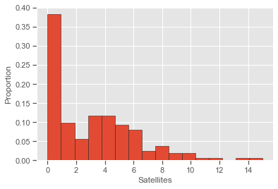
Negative binomial GLMs can be fitted in statsmodels. However, the dispersion parameter (1/k in formula, called alpha in Python) is not estimated (as in the glm.nb() function of the MASS package in R) and needs to be specified.
Thus, in practice a negative binomial GLM has to be fitted in two steps. First, we need to estimate the dispersion parameter and then fit the model. The estimation of the dispersion parameter can be done by a negative binomial model fitting in statsmodels.discrete.discrete model.
In order to estimate α correctly, we need to specify the design matrix of the GLM we want to fit. This stage yields correct estimates for the model parameters but not for their standard errors. In a second step, we re-fit the negative binomial GLM, setting the dispersion parameter equal to its estimate, derived in the first step.
# Step1
from statsmodels.discrete.discrete_model import NegativeBinomial

formula = 'sat ~ weight+C(color)'
model=NegativeBinomial.from_formula(formula, data=Crabs, loglike_method='nb2')
fit_dispersion=model.fit()
print(fit_dispersion.summary())
Optimization terminated successfully.
         Current function value: 2.155882
         Iterations: 24
         Function evaluations: 27
         Gradient evaluations: 27
                     NegativeBinomial Regression Results
==============================================================================
Dep. Variable:                    sat   No. Observations:                  173
Model:               NegativeBinomial   Df Residuals:                      168
Method:                           MLE   Df Model:                            4
Date:                Sun, 30 Oct 2022   Pseudo R-squ.:                 0.02798
Time:                        15:48:25   Log-Likelihood:                -372.97
converged:                       True   LL-Null:                       -383.70
Covariance Type:            nonrobust   LLR p-value:                 0.0002550
=================================================================================
                    coef    std err          z      P>|z|      [0.025      0.975]
---------------------------------------------------------------------------------
Intercept        -0.4263      0.559     -0.762      0.446      -1.522       0.670
C(color)[T.2]    -0.2528      0.351     -0.721      0.471      -0.940       0.435
C(color)[T.3]    -0.5219      0.379     -1.376      0.169      -1.265       0.222
C(color)[T.4]    -0.4804      0.428     -1.124      0.261      -1.319       0.358
weight            0.7121      0.178      4.005      0.000       0.364       1.061
alpha             1.0420      0.190      5.489      0.000       0.670       1.414
=================================================================================
#Step2
a = fit_dispersion.params[5]
fit = smf.glm('sat ~ weight + C(color)', family =sm.families.NegativeBinomial(alpha = a), data = Crabs).fit()
print(fit.summary())
                 Generalized Linear Model Regression Results
==============================================================================
Dep. Variable:                    sat   No. Observations:                  173
Model:                            GLM   Df Residuals:                      168
Model Family:        NegativeBinomial   Df Model:                            4
Link Function:                    log   Scale:                          1.0000
Method:                          IRLS   Log-Likelihood:                -372.97
Date:                Sun, 30 Oct 2022   Deviance:                       196.56
Time:                        15:48:25   Pearson chi2:                     155.
No. Iterations:                     7
Covariance Type:            nonrobust
=================================================================================
                    coef    std err          z      P>|z|      [0.025      0.975]
---------------------------------------------------------------------------------
Intercept        -0.4263      0.538     -0.792      0.428      -1.481       0.629
C(color)[T.2]    -0.2527      0.349     -0.725      0.468      -0.936       0.430
C(color)[T.3]    -0.5218      0.380     -1.373      0.170      -1.266       0.223
C(color)[T.4]    -0.4804      0.428     -1.122      0.262      -1.320       0.359
weight            0.7121      0.161      4.410      0.000       0.396       1.029
=================================================================================
The fit describes the tendency of the mean response to increase the weight, adjusting for color. Unlike the loglinear model, the color effect is no longer significant. The weight effect has standard error that increases from 0.068 in the Poisson model to 0.0161 in the negative binomial model.The estimated negative binomial dispersion parameters is 1.04.
Conclusion
