Fundamentals of Discrete Event Simulation(DES)
Introduction
In the last blog, we looked at SIS/SIR epidemic modeling using Discrete event simulation. This post will cover some fundamental concepts of Discrete Event Simulation, look at a few basic examples to develop an understanding, and end with a simulation of M/M/1 queuing model.
To get started, let’s look at an elementary example.Assume that we want to estimate the probability of observing the head
in an experiment of tossing a coin. We know that if the coin is not biased, then the likelihood of getting a head is 1/2.
We also know that if I toss the coin two or three times, we may not get exactly 1/2. We expect that if we keep tossing
the coin for a very long time, the average probability of getting heads will converge to 1/2.
Experiment
So let’s run the experiment 1000 times of tossing the coin, and we get 0.49 as the probability of getting head,
which is very close to our expectation of 1/2.
import random
import numpy as np
n = 1000
observed = []

for i in range(n):
    outcome = random.choice(['Head', 'Tail'])
    if outcome == 'Head':
        observed.append(1)
    else:
        observed.append(0)

print("Prob = ", round(np.mean(observed), 2))

Prob =  0.49 #Output
Let’s take a deeper look and see how the running mean was converging as the number of tosses increased.
n = 1000
observed = []

for i in range(n):
    outcome = random.choice(['Head', 'Tail'])
    if outcome == 'Head':
        observed.append(1)
    else:
        observed.append(0)

cum_observed = np.cumsum(observed)
moving_avg = []
for i in range(n):
    moving_avg.append(cum_observed[i] / (i+1))

x = np.arange(0, len(moving_avg), 1)

plt.plot(x, moving_avg)
plt.axhline(0.5, linewidth=2, color='black')
plt.title("Running Mean", fontsize=16)
plt.xlabel("Number of Tosses", fontsize=14)
plt.ylabel("Probabilty of Heads", fontsize=14)
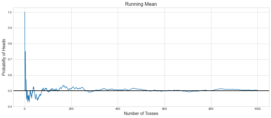
First, we can observe how the mean fluctuated widely around 0.5 but converged as the number of iterations increased.
So what we have done so far is that we ran a single experiment of tossing coin 1000 times and observed that it converges around 0.5. Now let’s repeat the experiment 1000 times with 10000 tosses in each experiment.
for i in range(1000):
    n = 10000
    observed = []

    for i in range(n):
        outcome = random.choice(['Head', 'Tail'])
        if outcome == 'Head':
            observed.append(1)
        else:
            observed.append(0)

    cum_observed = np.cumsum(observed)
    moving_avg = []
    for i in range(n):
        moving_avg.append(cum_observed[i] / (i+1))

    x = np.arange(0, len(moving_avg), 1)

    plt.plot(x, moving_avg)
    plt.axhline(0.5, linewidth=2, color='black')
    plt.title("Running Mean", fontsize=16)
    plt.xlabel("Number of Tosses", fontsize=14)
    plt.ylabel("Probabilty of Heads", fontsize=14)
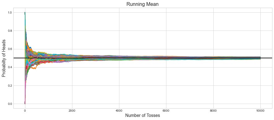
We can observe how each experiment in the initial start fluctuated and then later converged, similar to what we observed during a single experiment.
Law of Large Numbers
What we observed is an illustration of the Law of Large numbers. The Law of Large Numbers says that the average of the results obtained from a large number of trials should be close to the Expected Value and tends to become closer to the expected value as more trials are performed.
Transient and Steady Phase
Based on the above results, we can observe that each experiment goes through two phases, i.e., transient and steady. In the transient state, output varied wildly, and later, it converged in the steady phase. So while running simulation, it’s essential to run the experiments long enough to capture the Steady phase and not end it soon while it’s in the transient phase. Transient phase is also sometimes referred as the warm up period.
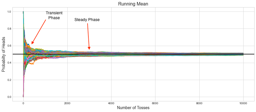
This will bring the question, how do we know how long is the transient phase, so we can discard the results observed in that state and only capture the steady state results. There are several method’s to detect that which you can refer in the paper EVALUATION OF METHODS USED TO DETECT WARM-UP PERIOD IN STEADY STATE SIMULATION. The simplest and yet an effective method is the Welch’s method.
Welch’s Method
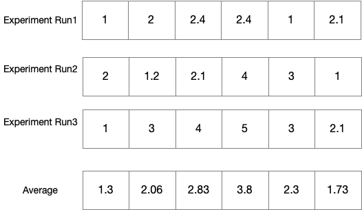
In simple words, Welch’s method says the following:
- Do Several Runs of the Experiment.
- Calculate the average of each observation across the runs.
- To smooth it further, calculate the moving average.
- Look at the graph visually and estimate the steady point from the graph.
n = 1000
Y = np.zeros(shape = (5, n))

def return_observations():
    observed = []

    for i in range(n):
        outcome = random.choice(['Head', 'Tail'])
        if outcome == 'Head':
            observed.append(1)
        else:
            observed.append(0)

    cum_observed = np.cumsum(observed)
    moving_avg = []
    for i in range(n):
        moving_avg.append(cum_observed[i] / (i+1))


    return moving_avg

for i in range(5):
    Y[i] =  return_observations()

Z = []
for i in range(n):
    Z.append(np.sum(Y[:, i])/ 5)

x = np.arange(0, n, 1)
plt.plot(x, Y[0], 'k--', linewidth=0.5, label="Y0")
plt.plot(x, Y[1], 'k--', linewidth=0.5, label="Y1")
plt.plot(x, Y[2], 'k--',  linewidth=0.5,label="Y2")
plt.plot(x, Y[3],  'k--', linewidth=0.5,label="Y3")
plt.plot(x, Y[4],  'k--', linewidth=0.5,label="Y4")

plt.plot(x, Z, linewidth=2,color='tab:red', label="Z")
plt.title("Running Mean", fontsize=16)
plt.xlabel("Number of Tosses", fontsize=14)
plt.ylabel("Probabilty of Heads", fontsize=14)
plt.legend()
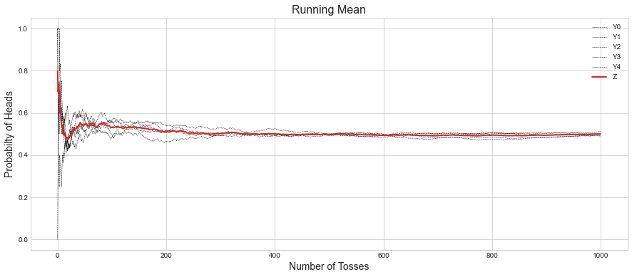
In the above plot, Red line is the average of the five runs at each iteration, and we can see that it’s steady somewhere between 300-400 iterations.
With this many coin tosses, I can’t let this go

Stochastic Process
Stochastic is a fancy word for Randomness. We observe Randomness every day in our life. The question is, are they random? Or is it because we lack a complete understanding of that process?. Without getting philosophical, to keep math simple, we attribute anything that we don’t understand to Randomness. Randomness can be known as different terms in TimeSeries analysis; we called that noise.
Coming back to the topic, A stochastic process is a collection of random variables whose observations are discrete points in time. At every instant of time, the state of the process is random. Since time is fixed, we can think of the state of the process as a random variable at that specific instant. At the time $t_{i}$, the state of the process is determined by performing a random experiment whose results are from the set of $\omega$. At the time $t_{j}$, the same experiment is performed to determine the next state of the process. This is the essence of the stochastic process.
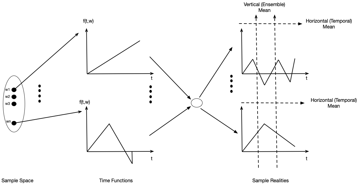
In the above diagram, the Sample space on the left is the set of outcomes that are mapped to a time function. The time functions are mixed to get sample reality.
If the above seems mouthful, hopefully, the following example will help. The Marvels Multiverse universe is the best analogy that always comes to mind while thinking of the Stochastic Process. Remember this scene from Infinity Wars, where Doctor Strange looked at 14 million different realities, and in only one reality, the outcome of Avengers winning was one.

So tying this back to Stochastic Process, In this case, The set of outcomes were two, Avengers Winning and Thanos Winning. This is a sample space of outcomes. Each outcome is related to some set of actions performed. Those actions are mixed to form a sample reality.
Another key concept is that a Stochastic process can have two means, Vertical mean, also known as Ensemble mean. Ensemble mean is calculated vertically over all realities. A horizontal mean is the mean of a single sample reality. As you can notice, getting an Ensemble mean requires running all possibilities that may or may not be feasible. But the good thing is that a horizontal mean can be used to approximate vertical mean.
A dynamic system can be viewed as a Stochastic Process. When system is simulated, each simulation run represents an evolution of the system along the path in the state space. The data generated and collected along the trajectory in the state space is used to estimate the measurements of interest.
A Dynamic system is called Ergodic system if the Horizontal mean converges to the Vertical mean.
Simulating M/M/1
Now let’s look at the same concepts visited above with example simulations for the M/M/1 queuing system to figure out the average delay. Assume that we have 100K packets to serve; the Poisson process is used to model both packet’s arrival and service rate. Both arrival and service rates are between 1 to 3 packets per unit of time.
We know that in a queuing system, the delay will increase if the service rate is lower than the arrival rate (more packets are coming in, and fewer packets are going out).
def average_delay(lamda, mu):
    NUM_PKTS = 100000 # Number of Packets
    count = 0 # Count
    clock = 0 # Clock
    N = 0

    ARR_TIME = expovariate(lamda)
    DEP_TIME = np.inf

    ARR_TIME_DATA = []
    DEP_TIME_DATA = []
    DELAY_DATA = []

    while count < NUM_PKTS:
        if ARR_TIME < DEP_TIME:
            clock = ARR_TIME
            ARR_TIME_DATA.append(clock)
            N = N + 1
            ARR_TIME = clock + expovariate(lamda)
            if N == 1:
                DEP_TIME = clock + expovariate(mu)
        else:
            clock = DEP_TIME
            DEP_TIME_DATA.append(clock)
            N = N - 1
            count = count + 1
            if N > 0 :
                DEP_TIME = clock + expovariate(mu)
            else:
                DEP_TIME = np.inf

    for i in range(NUM_PKTS):
        d = DEP_TIME_DATA[i] - ARR_TIME_DATA[i]
        DELAY_DATA.append(d)

    return (round(np.mean(DELAY_DATA), 4))

df = pd.DataFrame(columns=['mu', 'lamda', 'delay'])
lamda_range = np.arange(1, 3, 0.1)
mu_range = np.arange(1,3,0.1)
i = 0
for mu in mu_range:
    for lamda in lamda_range:
        df.loc[i] = [mu, lamda, average_delay(lamda, mu)]
        i+=1
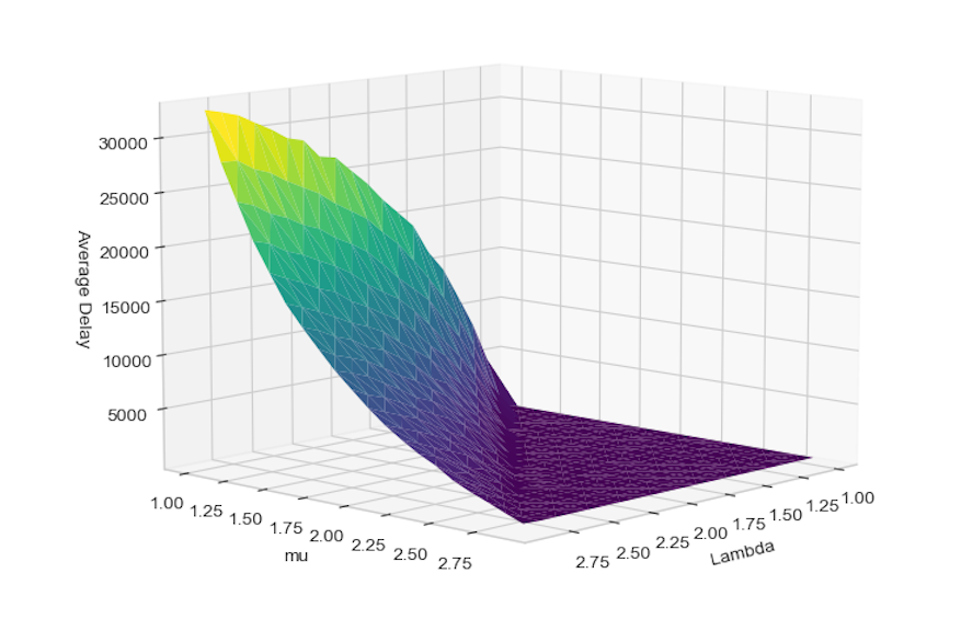
If we look at the plot, we can see that the average delay is flat surface indicating low delay wherever packet arrival rate (lambda) is lower than service rate (mu). Delay shoots up whenever the service rate is lower than the Arrival rate, as indicated by the rising surface.
Conclusion
In this blog, we covered some fundamental concepts of Discrete event simulation. Then we applied that to simulate M/M/1 queuing model. We will try to cover event graphs and model a simple Automatic Repeat Request(ARQ) protocol in a future post.