ECMP is crucial for scaling and performance in modern data centers and wide-area networks, which rely on hash-based path selection. It leverages path diversity and keeps a flow’s packets on the same path, preventing reordering with useful properties like stateless operation and no reordering.

While simple and widely used, ECMP has some limitations. For example, it does not always distribute traffic evenly across all available paths. However, due to its ease of hardware implementation, ECMP remains the predominant approach. The core enabler for ECMP is hashing, which allows packet-by-packet path selection in a distributed manner across switches. ECMP limitations have also started getting more attention with the surge in building GPU clusters but fabrics suffer from Poor hashing due to a lack of flow entropy.

In this post, we’ll dive into ECMP and use statistical analysis to better understand the limitations.

Introduction

Here is a simplified explanation of how the lookup process functions. We aim to perform a prefix lookup that directs us to a specific ECMP Group listed in the ECMP group table. Each of these ECMP groups contains ECMP member counts for the ECMP group. A hash function takes Packet fields i.e. our typical five tuple (Source and Destination IP,Source and Destination Port, Protocol) and a seed (to avoid Hash polarization) as an Input and produces a Hash $H$. If there are $n$ members in an ECMP group, a specific member within an ECMP member set is selected using $H \mod{n}$.

Hash Function

A hash function maps a bit vector onto another, usually shorter, bit vector. Typically the $m > n$ which is why sometimes hash functions are also called compression functions.

All good hash functions share the property of collision avoidance, which means that the desired behavior is for unique inputs to provide unique outputs. However, If the length of the vector is greater than the length of the output vector, it’s impossible to avoid all collisions because the set of input vectors will be of greater order than the set of output vectors. Since collisions can not be avoided, the goal is to minimize their likelihood given two arbitrary input vectors.

The most commonly used Hash function implemented in hardware are XOR and CRC or their variants for ECMP hashing. I am going to focus on CRC variants for illustrations.

Polynomials

A polynomial is a single-variable function made up of addition, multiplication, and exponentiation operations. It can be expressed in the form:

Here, $c_{n}$ are the coefficients, and each power of $x$ marks a different term. For example, $x^5 + 3x^2 + 2x + 5$ is a polynomial. You can easily add or subtract polynomials by combining the coefficients of the same terms. If a term is missing in one polynomial, it’s treated as if it has a coefficient of zero. Example of addition:

If you plug in $x=3$, both expressions will give you 192.

Multiplying polynomials involves multiplying each term in one polynomial with every term in the other and then combining like terms. Example:

Polynomial division can also be carried out, even using bits for simpler calculations. You convert the polynomials to binary and divide bit by bit, carrying over the remainder to the next bit, until you reach zero for the dividend.

CRC Hash example

Let’s say you want to divide $x^3 + x + 1$ by $x^2 + 1$. In binary, these become $1011$ and $101$ respectively. Because our divisor $x^2+1$ is of degree two, we will add two zeros at the end of $101100$ and perform the division which gives us a remainder of 1.

        1001  
    --------  
101 ) 101100  
     ⊕101  
     ----  
         100  
         101  
         ---  
           1

The divisor used in our example, $101$, is commonly called the generator polynomial, and $101100$ represents the message we’re working with. The resulting CRC hash, in this case, is $01$, which is the remainder left after division. This process illustrates how a CRC hash is created. CRC16 or CRC32 are common variants which are generally implemented.

Generator Polynomial

In the example above, we had a message for which we wanted to create a hash in bit form. However, we can’t just pick any divisor for this calculation. The divisor, or the generator polynomial, must be a primitive polynomial. This means it can’t be divided by any polynomial with a lower degree than itself. If you’re curious to learn more about the properties of primitive polynomials, you can explore the topic further at COMPUTING PRIMITIVE POLYNOMIALS.

Some well known generator polynomials used for CRC16 and CRC32:

CRC-16    0x8005     x^16 + x^15 + x^2 + 1
CRC-CCITT 0x1021     x^16 + x^12 + x^5 + 1
CRC-DNP   0x3D65     x^16 + x^13 + x^12 + x^11 + x^10 + x^8 + x^6 + x^5 + x^2 + 1
CRC-32    0x04C11DB7 x^32 + x^26 + x^23 + x^22 + x^16 + x^12 + x^11 + x^10 + x^8 + x^7 + x^5 + x^4 + x^2 + x^1 + 1

Another example

Let’s say I have four different interfaces, and any one of them is chosen based on the hash based on a set of five tuples. I am going to randomly generate ten sessions using source IP addresses that range from $192.168.1.10 - 192.168.1.20$ and source ports that range between $49512 - 65535$. I calculate the hash using a generator polynomial of $0\text{x}1021$ . After computing the hash, we calculate the outgoing interface using $\text{H} \mod \text{n}$.

def crc16_custom(data: str, polynomial=0x1021, initial_value=0xFFFF) -> int:
    crc = initial_value
    for byte in data.encode('utf-8'):
        crc ^= byte
        for _ in range(8):
            if crc & 1:
                crc = (crc >> 1) ^ polynomial
            else:
                crc >>= 1
    return crc & 0xFFFF

for i in range(10):
    src_ip = f'192.168.1.{random.randint(10, 20)}'
    dst_ip = '172.16.2.50'
    src_port = random.randint(49512, 65535)
    dst_port = 22
    protocols = 6
    five_tuple = (src_ip, dst_ip, src_port, dst_port,protocols)

    # Convert the 5-tuple to a single string
    five_tuple_str = ''.join(map(str, five_tuple))

    # Compute the CRC16 hash using custom implementation
    crc16_custom_hash = crc16_custom(five_tuple_str)
    print(f"{five_tuple}, Interface: {crc16_custom_hash%4+1}")

('192.168.1.11', '172.16.2.50', 62660, 22, 6), Interface Selected: 1
('192.168.1.18', '172.16.2.50', 56763, 22, 6), Interface Selected: 4
('192.168.1.14', '172.16.2.50', 50661, 22, 6), Interface Selected: 2
('192.168.1.19', '172.16.2.50', 61342, 22, 6), Interface Selected: 2
('192.168.1.17', '172.16.2.50', 64823, 22, 6), Interface Selected: 3
('192.168.1.14', '172.16.2.50', 49870, 22, 6), Interface Selected: 2
('192.168.1.15', '172.16.2.50', 63685, 22, 6), Interface Selected: 1
('192.168.1.13', '172.16.2.50', 63333, 22, 6), Interface Selected: 1
('192.168.1.15', '172.16.2.50', 61262, 22, 6), Interface Selected: 3
('192.168.1.13', '172.16.2.50', 50180, 22, 6), Interface Selected: 3

Dynamics between Network Flows and ECMP Paths

It’s commonly understood that if we increase the number of ECMP paths while keeping the number of flows constant, will create inefficiencies, primarily due to the constraints of hashing algorithms. This can be observed by generating unique flows, calculating the CRC hash, and tally the number of flows assigned to each interface. Subsequently, we can increase the number of flows and again count the number of flows assigned to each interface.

However, to accurately compare the variability in flow distribution across interfaces as we increase the number of flows, we require a metric that is stateless. Traditional measures like standard deviation or variance wouldn’t be suitable here, as they only quantify the deviation within a single distribution. For this scenario, the Coefficient of Variation serves as a more appropriate metric.

Coefficient of Variation (CV)

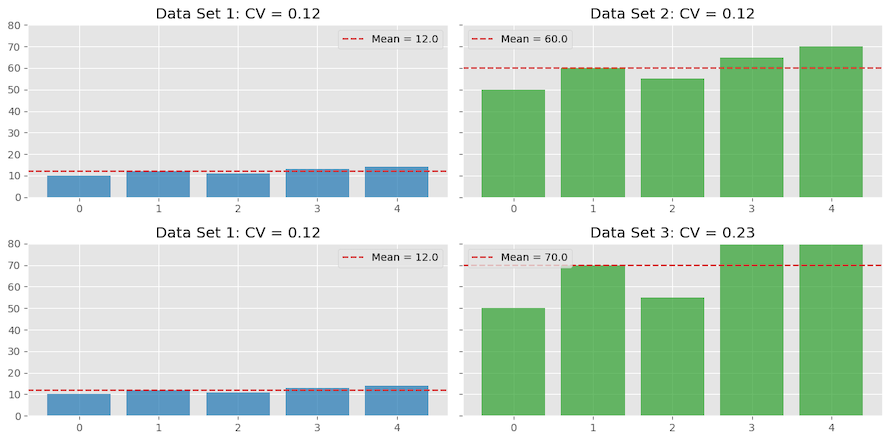
The Coefficient of Variation is a unitless measure that shows how spread out data is relative to its mean. For example, consider two runners, Alice and Bob. Alice runs 5 miles daily with a 1-mile variability, and Bob runs 10 miles with a 2-mile variability. While Bob’s variability is larger, both have a same CV of 20%, indicating their running distances are equally variable relative to their averages. The Coefficient of Variation allows for comparing the relative variability of different data sets, regardless of scale or units.

In another example comparing three data sets, Data set 1 and Data set 2 both have the same variability of 12% (CV of 0.12). However, when comparing Data set 1 with Data set 3, the latter shows higher variability.

Variability in Flow Distribution Across Specified ECMP Paths

The graph below illustrates the number of flows assigned on each interface for varying numbers of flows—250, 500, 1K, 5K and 10K—across 16 ECMP paths. I am using CRC-32 with a generator polynomial 0xEDB88320. We can see that the Coefficient of Variation (CV) score decreases as the number of flows increases indicating that variability decreases when the number of flows increases. This means flow assignment tends more towards uniform distribution as the number of flows increase.

I’ve created separate plots for 250 and 500 flows, as their scale made them difficult to discern clearly when combined with the others.

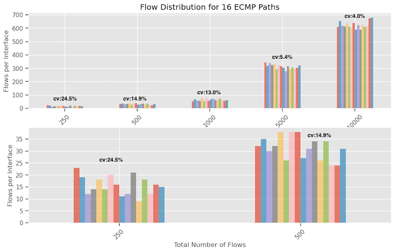
Below, the data indicates a zero-collision rate during hash generation using the five-tuple inputs. Despite this, the distribution across links is not uniform.

No. of Flows: 250, No. of Links 16, Collision Rate 0.0
No. of Flows: 500, No. of Links 16, Collision Rate 0.0
No. of Flows: 1000, No. of Links 16, Collision Rate 0.0
No. of Flows: 5000, No. of Links 16, Collision Rate 0.0
No. of Flows: 10000, No. of Links 16, Collision Rate 0.0

This discrepancy arises from the inherent probabilistic nature of the $\text{H}\mod \text{n}$ operation. When applying this operation to a CRC hash value, the potential remainders range from $0$ to $n-1$, each with an equal likelihood of occurrence. For instance, with a 32-bit CRC hash and $n=4$, the possible remainders—0, 1, 2, and 3—are each likely to occur 25% of the time. As $n$ increases, the chance of any specific remainder occurring diminishes to $1/n$. The $\text{mod}$ operation essentially maps the broad spectrum of CRC hash values into a confined range from 0 to $n-1$, and it is this compression that leads to collisions. We will look into the probabilistic distribution aspects later.

Flow Distribution Variations with Changing ECMP Paths and Fixed Flows

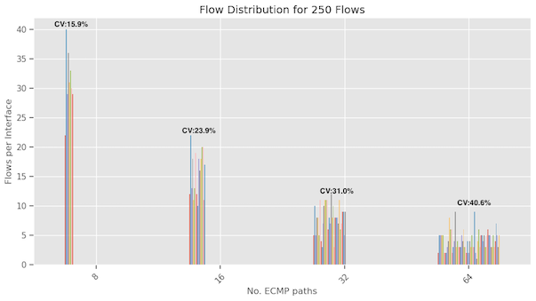
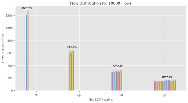
Previously, we examined how the distribution of flows varied across interfaces when we increased the number of flows, keeping the ECMP paths fixed at 16. Now we’re keeping the number of flows constant and varying the number of ECMP paths, exploring counts of 8, 16, 32, and 64.

The following graphs display results for both 250 and 10,000 flows. In both cases, we observe that as the number of ECMP paths increase, the variability in flow assignments also increases, as indicated by the Coefficient of Variation score. This should be intuitive as imagine if we have only one interface, then there will be no variability and as we increase the ECMP paths, the probabilistic aspects will come and variability will increase.

We observe that the variability in flow distribution is more significant for 250 flows than 10,000 flows when assessed on a specific ECMP path. This observation aligns with the findings from the previous section. It offers insights into why reduced flow diversity results in suboptimal interface utilization.

Theoretical Analysis of Flow Distribution Across ECMP Paths

Let’s delve into the theoretical perspective of how flows are distributed across ECMP paths. Think of this scenario as a ‘balls and bins’ problem, where each ball has an equal chance of landing in any given bin. In our context, the balls represent network flows, and the bins symbolize the ECMP paths. We can then compute the theoretical probability of a flow being assigned to a particular ECMP path.

To better grasp this concept, consider a basic experiment where 16 balls are randomly allocated among four bins. You can see the numbers of balls assigned to each bin and it is never perfect.

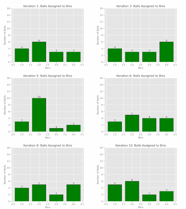
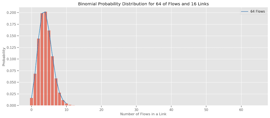
We can model this behavior using Binomial distribution under the assumption that each flow has an equal chance of being assigned to each ECMP path (i.e., $1/n$ where $n$ is the number of ECMP Paths). Given $n$ number of links and $m$ number of flows, we can calculate the probability of $k$ flows being assigned to ECMP path is:

Here, $\mathrm{C}_{k}^{m}$ represents the number of combinations of $m$ flows taken $k$ at a time, and $P(k)$ is the probability of $k$ flows being assigned to a specific link.

This plot shows the probabilities of $k$ flows out of 64 flows landing on 16 links. We can see the highest probability is of landing 4 or 5 flows on a link but others are not zero.

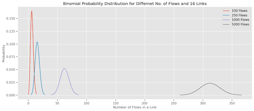
Here is the distribution for different number of flows for 16 links. One issue with this plot is that this is deceiving due to the scale of number of flows being so different. Ideally we would have expected as that the number of flows increase, the probability bands to get more tighter showing less variability like we saw in our earlier experiments. But I think that’s a visual artifact.

When we have more flows (larger n), the standard deviation increases in absolute terms but decreases relative to the mean (which is $n \times p$). This makes the distribution look narrower when plotted on the same scale.

We could normalize the binomial distribution for different numbers of flows getting assigned to 16 links. Have x-axis represents the proportion of flows in a single link (normalized by the total number of flows), and the y-axis represents the probability of that occurring.

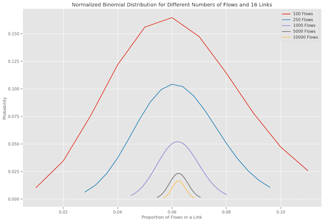
In this normalized view, we can observe the following:

1. As the number of flows increases, the distribution becomes narrower.
2. For a smaller number of flows (e.g., 100 or 250), the distribution is wider, indicating higher variability in the number of flows that might get assigned to a specific link.
3. For a larger number of flows (e.g., 5000 or 10000), the distribution is more focused around the expected value, indicating lower variability.

The phenomenon of the distribution becoming narrower with a higher number of flows is more evident in the normalized plot. This is in line with the characteristics of the binomial distribution; as the sample size (number of flows) increases, the distribution tends to become narrower, converging towards its expected value. This is a manifestation of the Law of Large Numbers.

Additional Resources for Deeper Exploration

Here are some additional resources which I wasn’t able to delve into but are worth exploring for those interested in going further.

1. Birthday Paradox
2. Google recent paper around there proposal of using different hash algorithms and coloring
3. Hashing Linearity Enables Relative Path Control in Data Centers

References

1. Birthday Paradox
2. Hashing Design in Modern Networks: Challenges and Mitigation Techniques
3. Hashing Linearity Enables Relative Path Control in Data Centers
4. Binomial distribution
5. Law of large numbers
6. Coefficient of Variation
7. CRC