Introduction

You may or may not have already heard about the Five Number summary for a dataset. It’s basically a set of descriptive statistics for a given dataset, which provides an idea about the dataset. Those are:

1. Minimum
2. First quartile
3. Median
4. Third quartile
5. Maximum

Similarly, there are specific statistics about topology, which gives an idea about any network topology. The ones which I think the most essential are:

1. Density and Sparsity
2. Average Degree
3. Assortativity
4. Average Path Length
5. Clustering Coefficient

Sample Topology

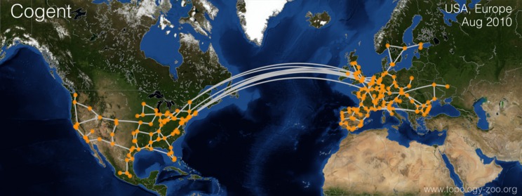
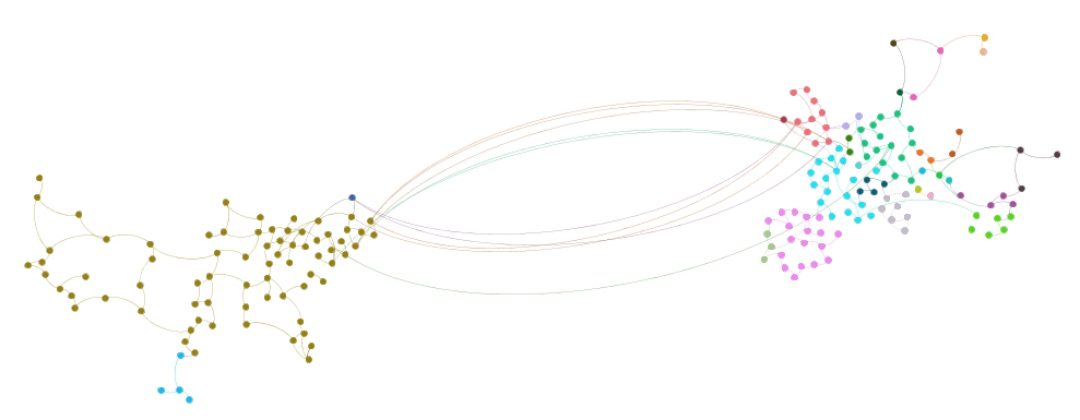
We will be using Cogent topology, which is publicly available here to follow along with our examples. The map represents the nodes in US + Mexico, and European countries.Each node color represents a specific country.

Graphml version

You may have already noticed that in the graph, each city is represented as a Node. In reality, any city will have many routers, which will make the topology a lot bigger and more attractive. For our purposes, the current topology abstraction provides the right balance where it’s not huge to overwhelm the reader but big enough to keep things interesting.

Five Number Summary

Density and Sparsity

A Graph consists of nodes and links connecting those nodes. An obvious thing to say is that the maximum links a graph can have are bounded by its nodes. This means the maximum number of links a network can have can be given by the number of nodes. A Complete Network is the one which has all possible pair of nodes connected by links.

A maximum number of links in an Undirected network with \(N\) nodes, can be given by:

We know what the max links a graph can have, but the actual links can be that or less. The links which actually exists in the network is known as the density of the network. A Complete network will have maximal density. If the network’s density is much smaller than maximal links, we called this sparsity. Most of the networks we see in real life are sparse.

Density of the Network is given by:

We can substitute \(L_{max}\) in the equation and get

In a complete network, \(L = L_{max}\) which means density d = 1. In a sparse network, \(L << L_{max}\) and therefore \(d << 1\) (symbol \(<<\) means much less than).

As a network grows, nodes will increase, which will increase the number of Links. Hence we can say that the number of links is a function of the number of nodes. If the number of links grows proportionally to the number of nodes $(L \sim N)$ or slower, then we can say that the network is sparse. If the number of links grows faster e.g. quadratic or cubic growth \((L \sim N^2 or N^3)\), then we say that the network is dense.

Let’s look at our sample cogent topology.

import networkx as nx
G = nx.read_graphml(filename)
NODES = len(G.nodes())        // 197
LINKS = len(G.edges())        //245
MAX_LINKS = (197* (197-1))/2  //19306
Density = 245/19306           //0.0126

We have Nodes = 197, Links = 245 and the density = 0.0126. This indicates that our topology is sparse in nature.

Degree

A degree of a node is the number of links or neighbors. We will use \(k_{i}\) to denote the degree of node \(i\). A node with no neighbors will have degree = 0 and is called Singleton. The average degree of a network is defined as the sum of degree of all nodes divided by the number of nodes N.

Let’s look at the average degree of nodes in our Cogent topology.

sum([d for (n, d) in nx.degree(G)]) / G.number_of_nodes() // 2.48

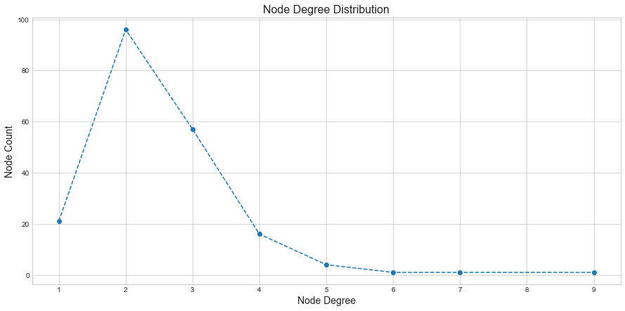
The average node degree for our cogent topology is around 2.48. This means on an average most nodes are connected to 2-3 neighbors. Let’s plot the degree distribution of our graph and see how it looks like:

.

You can observe that the maximum nodes have degree = 2 (peak), and it has a thin tail on the right with very few nodes with a high degree of 6,7,8 and 9.

Average Weighted Degree

In our simple case, all links between nodes were equal. We didn’t provide importance to any given link over another. But some links may be more important than others, and we may provide the weights to them (e.g., IGP Cost/Link Capacity). The weighted degree of a node is like a degree but ponderated by the weight of each edge. For instance, a node with 4 edges with weight 1 each(1+1+1+1) is equal to a node with 2 edges with weight 2 (2+2).

Assortativity

Assortatvitiy is a property of the network where nodes with similar features are connected together. We see this property in social networks all the time where people with similar interests are friends a.k.a connected to each other. This is also captured by the popular saying that “birds of a feather flock together” and technically it’s called as Homophily.

We know that a degree is a property of a Node. Assortativity based on degree is called degree assortativity. In this high degree nodes are connected to high degree nodes and low degree nodes tends to connect low degree nodes. This type of network is called Assortative. If the high degree nodes tend to connect to low degree nodes and vice versa then that network is called dissasortatvie.

There are two ways to measure degree assortatvity of a network, both based on measuring the correlation between degrees of neighbor nodes.

One way to measure network assortativity is by assortativity coefficient, defined as the pearson correleation between the degrees of pairs of linked nodes. If the coefficient is positive, then the network is assortative and disassortative if it’s negative.

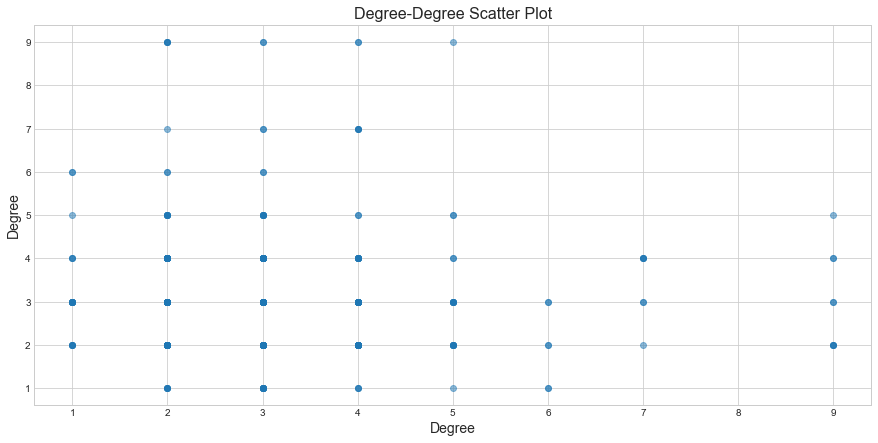
If we look at the below degree-degree scatter plot of our Cogent Topology, we can observe that most low degree nodes are connected to other low degree nodes but also connected to few high degree nodes. The shades indicate the density, it’s not very conclusive but there are darker shades between low degree nodes.

It seems like our network may be slightly assortative—the degree assortativity coefficient= 0.019, which is a positive value indicates that our topology is slightly assortative but not much due to the value closer to zero.

nx.degree_assortativity_coefficient(G) //0.019

The second method is based on measuring the average degree of the neighbors of node i

where \(a_{ij} = 1\), if i and j are neighbors and 0 otherwise. We then define K-nearest neighbors function \(K_{nn}(k)\) for nodes of a given degree \(K\) as the avg. degree of k_nn(i) across all nodes with degree k. if \(K_{nn}(k)\) is an increasing function of k then high degree nodes tend to be connected to high degree nodes; there the netowork is assortative, if \(K_{nn}(k)\) decreases with k, the network is disassortative.

Average Path Length

It’s possible to define an aggregate distance measure for the entire network by using the shortest path length as a measure of distance between nodes. The Average Shortest Path Length is obtained by averaging the shortest path lentgh across all pair of nodes.

Formally the Average Shortest Path Length for an undirected graph is given by

where \(l_{ij}\) is the shortest path length between nodes \(i\) and \(j\) and \(N\) is the number of the nodes.

The diameter of the network is the max shortest path length across all pairs.

The Average shortest path length for our example topology is 10.5 hops.

nx.average_shortest_path_length(G) // 10.5
nx.diameter(G) // 28

Small World Property

A small world property is a popular notion that social distances are short on average. For example, If I just consider the network engineer population, If I have to guess, then most of the engineers are either 3 or 4 connections away from any other engineer. Some famous folks will act as Hubs, and most folks will be connected to them.

This is also known as “six degrees of seperation” where the idea is that all people on average are six or fewer connections away from each other. This also means that the circle of our friends of friends is vast than we think. We often say this when we run into people again or know someone in common that it’s a small world.

We can see, if the real-life networks exhibit this small world property or not. But before we go further, let’s say if the network only consists of 10 nodes and the average path length is around 5 or 6, is that a short path in the network? What if the network consists of 1 million nodes, and the average path length is around 5 or 6. Is that a short path in the network?.

It turns out that when our Average Shortest Path length grows slowly with the size of the network, then we consider the path lengths to be short. We can express this mathematically.

Clustering Coefficient

A clustering coefficient is the average probability that two friends of a node are also friends. In other words, It’s the ratio between the number of triangles that include the node, and the maximum number of triangles in which the node can participate.

It’s formally given as:

where \(\tau (i)\) is the number of triangles involving i. The Clustering Coefficient of the entire network is the average of the clustering coefficients of its nodes:

Nodes with degree K < 2 are excluded when calculating the average clustering coefficient.

A low clustering coefficient means that the network has few triangles, while a high clustering coefficient means that the network has many triangles.

nx.average_clustering(G) \\ 0.016

The clustering Coefficient for our Topology is low indicating little to no clusters in our topology.

Summary

We looked at some essential properties of Network Topologies. Five Number summary for our Sample Topology

1. Desity: 0.0126
2. Avg Degree: 2.48
3. Assortativity Coefficient: 0.019
4. Avg Path length: 10.5
5. Clustering Coefficient: 0.016

These properties can be used to assess various network topologies and understand the deep structure while doing topology design. In the next upcoming posts, we will look at more network science aspects, meanwhile, how does the above five summary number look like for your network?