Two roads diverged in a wood, and I–I took the one less traveled by, And that has made all the difference.- Robert Frost

Disjoint Path routing problems involve finding multiple paths between a source and a destination pair without any shared components. There are different types of disjoint paths, each with specific requirements. For example, link disjoint paths ensure that the paths do not have any common links, while node disjoint paths guarantee that the paths do not share any common nodes. SRLG disjoint paths are another variation, where the paths do not share any common risk groups.

These problems are commonly addressed to ensure network reliability, load balancing, and congestion reduction. The first problem we will examine is the MIN-SUM problem, which aims to determine a set of disjoint routes with the lowest overall cost. To solve this issue, we will look at integer linear programming (ILP). Afterwards, we will explore the MIN-SUM problem in the context of networks with shared risk link groups (SRLGs) and present corresponding solutions.

Basic Disjoint Problem

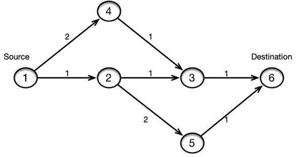
Let’s say our problem is to find a simple link disjoint paths between a given source and destination. One of the common ways we hear to do in a naive way is to find the shortest path first, remove the edges on the shortest path and run Dijkstra again to find another shortest path. The Problem with this approach is that it’s not always possible to find the diverse paths.

For example, in this topology the shortest path between 1 and 6 is 1->2->3->6 and when we remove these edges to find the next shortest path, we end up having no paths between 1 and 6. We can use Integer Linear Programming (ILP) to solve this problem, which is a more constrained version of Linear Programming (LP).

Integer Linear Programming

ILP (Integer Linear Programming) is a type of linear programming where one or more of the decision variables must be integers. This makes ILP a more complex optimization problem compared to LP (Linear Programming), which only deals with continuous variables. In ILP, the solution not only needs to satisfy the linear constraints, but it must also be an integer coordinate. This requirement significantly reduces the set of feasible solutions compared to an LP.

Let’s look at a simple problem. Assume that we have an objective function to maximize $5x_{1}+4x_{2}$ with constraints listed below.

If we plot the above graphically, we can see the feasible region of the problem as a 2D projection.

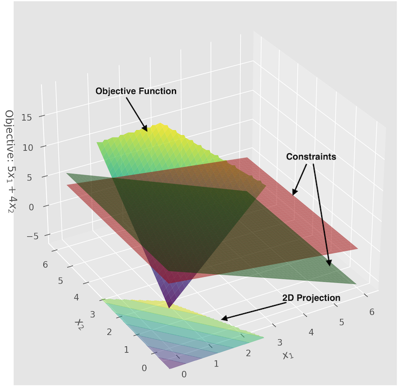
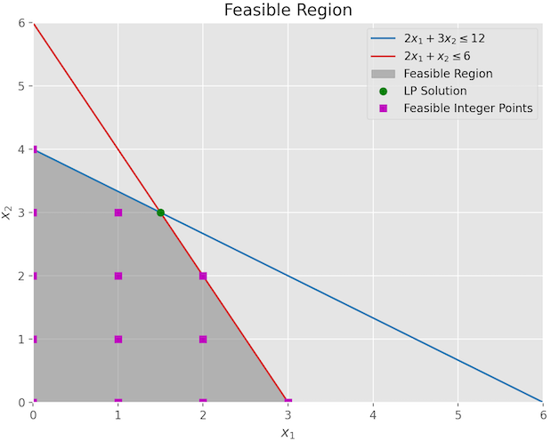
The plot below shows the 2D view with the feasible region of the problem space shaded in gray. If we wanted an the LP solution then the green dot would have been our optimal solution i.e. $x_{1} = 1.5, x_{2} =3$. This gives us $5 \times 1.5 + 4 \times 3 = 19.5$ as the answer for objective function.

All the square dots shown on the plot represent the potential solutions for the ILP solution. You’ll notice that they are located either on the boundaries or inside the feasible region. In this specific problem, the optimal ILP solution is at $x_{1}=0,x_{2}=4$. This gives us $5 \times 0 + 4 \times 4 = 16$ for the objective function using ILP. The optimal solution of ILP $\le$ optimal solution of LP.

The ILP problems are hard to solve and also known as NP-hard problem. We solve ILP problems using heuristics and commonly used techniques are Branch and Bound and Cutting planes.

ILP Formulation of Disjoint Path Problem

Let’s assume that we want to find K disjoint paths from a source node p to a destination node q. What we want is that the sum of the cost of all the paths to be minimized, in that way we aren’t finding disjoint paths which are taking sub-optimal paths.This is quantified as the sum of the costs of all paths, where each path’s cost is the sum of the costs of its links.

we can write the objective function as

Here $d_{ij}$ is the cost of link $(i,j)$ and $x_{ij}^k$ is a binary variable which indicates if link $(i,j)$ is used in path k or not.

As always we need the Flow conservation constraint to ensure that each path k behaves as a flow network, where the amount entering a node (except for the source and destination) must equal the amount leaving it.

We also need to add path definition constraints to ensure that for each path k, there is exactly one incoming edge to the destination and one outgoing edge from the source. $\sum_{j:(p,j)\in E}x_{pj}^k = 1$ and $\sum_{j:(j,q)\in E}x_{jq}^k = 1$ for all path $k$.

For the disjointness constraint, example link disjoint constraint we need to make sure no link is used by more than one path k. $x_{ij}^{k1} + x_{ij}^{k2} \le 1$ for all links $(i,j)$ and all pairs of paths $(k1, k2)$, $k1 \ne k2$. If a link is used by one path, $x_{ij}^k$, for that path and link will be 1, forcing to be 0 for all other paths.

The variables $x_{ij}^k$ are binary integers(0 or 1). This defines the problem as an integer linear programming problem. Now let’s convert this problem into code. Here is the relevant snippet which converts our original graph problem

# Define the source and destination nodes
source = 1
destination = 6

# Define the number of disjoint paths
K = 2

# Create the problem
prob = LpProblem("Disjoint_Paths_Problem", LpMinimize)

# Create decision variables
x = {}
for k in range(1, K+1):
    for (i, j, key) in G.edges(keys=True):
        x[i, j, key, k] = LpVariable(f"x_{i}_{j}_{key}_{k}", cat=LpBinary)

# Set the objective function
prob += lpSum(G[i][j][key]['cost'] * x[i, j, key, k] for k in range(1, K+1) for (i, j, key) in G.edges(keys=True))

# Set the constraints
# Flow conservation constraints
for k in range(1, K+1):
    for i in G.nodes:
        if i == source:
            prob += lpSum(x[i, j, key, k] for (i, j, key) in G.out_edges(i, keys=True)) - lpSum(x[j, i, key, k] for (j, i, key) in G.in_edges(i, keys=True)) == 1
        elif i == destination:
            prob += lpSum(x[i, j, key, k] for (i, j, key) in G.out_edges(i, keys=True)) - lpSum(x[j, i, key, k] for (j, i, key) in G.in_edges(i, keys=True)) == -1
        else:
            prob += lpSum(x[i, j, key, k] for (i, j, key) in G.out_edges(i, keys=True)) - lpSum(x[j, i, key, k] for (j, i, key) in G.in_edges(i, keys=True)) == 0

# Disjoint path constraints
for (i, j, key) in G.edges(keys=True):
    prob += lpSum(x[i, j, key, k] for k in range(1, K+1)) <= 1

# Solve the problem
prob.solve(PULP_CBC_CMD(msg=0))

# Answer
Minimum total cost: 8.0
{'Path 1: (1, 2) -> (2, 5) -> (5, 6)'}
{'Path 2: (1, 4) -> (4, 3) -> (3, 6)'}

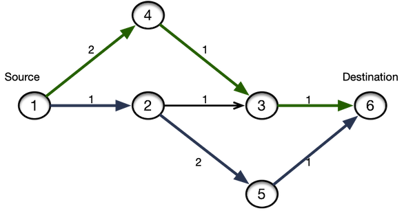
The disjoint paths we get are 1->2->5->6 and 1->4->3->6 and the total cost for the paths is 8.

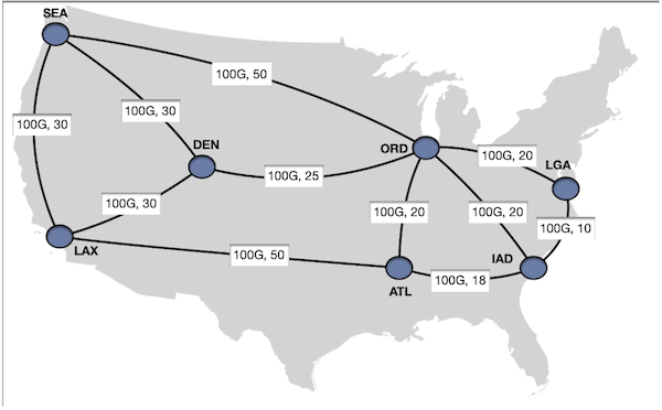
Now let’s use our toy graph which we have been using to find disjoint paths from sea to iad. We will also add a capacity constraint such that the links traversed by the paths also meets the capacity constraint.

Relevant code snippet.

# Define the number of disjoint paths
K = 2
# Create the problem
prob = LpProblem("Disjoint_Paths_Problem", LpMinimize)

# Create decision variables
x = {}
for k in range(1, K+1):
    for (i, j, key) in G.edges(keys=True):
        x[i, j, key, k] = LpVariable(f"x_{i}_{j}_{key}_{k}", cat=LpBinary)

# Variables for the selection of edges for each disjoint path
edge_vars = LpVariable.dicts("Edge", [(i, j, key, k) for i, j, key in G.edges(keys=True) for k in range(K)], 0, 1, cat='Binary')


# Variables for the flow on each edge for each demand and disjoint path
flow_vars = LpVariable.dicts("Flow", [(src, tgt, i, j, key, k) for src, tgt, _ in demands for i, j, key in G.edges(keys=True) for k in range(K)], 0)


# Objective function: minimize the total cost of the disjoint paths
prob += lpSum(G[i][j][key]['cost'] * edge_vars[i, j, key, k] for i, j, key in G.edges(keys=True) for k in range(K))


# Set the constraints
# Flow conservation constraints
for src, tgt, amt in demands:
    for k in range(K):
        for node in G.nodes():
            if node == src:
                prob += lpSum(flow_vars[src, tgt, node, j, key, k] for _, j, key in G.out_edges(node, keys=True)) - lpSum(flow_vars[src, tgt, i, node, key, k] for i, _, key in G.in_edges(node, keys=True)) == amt
            elif node == tgt:
                prob += lpSum(flow_vars[src, tgt, i, node, key, k] for i, _, key in G.in_edges(node, keys=True)) - lpSum(flow_vars[src, tgt, node, j, key, k] for _, j, key in G.out_edges(node, keys=True)) == amt
            else:
                prob += lpSum(flow_vars[src, tgt, node, j, key, k] for _, j, key in G.out_edges(node, keys=True)) - lpSum(flow_vars[src, tgt, i, node, key, k] for i, _, key in G.in_edges(node, keys=True)) == 0


# Disjoint path constraints
for i, j, key in G.edges(keys=True):
    prob += lpSum(edge_vars[i, j, key, k] for k in range(K)) <= 1


# Capacity constraints
for i, j, key in G.edges(keys=True):
    prob += lpSum(flow_vars[src, tgt, i, j, key, k] for src, tgt, _ in demands for k in range(K)) <= G[i][j][key]['capacity']


# Link flow and edge selection constraints
for src, tgt, _ in demands:
    for i, j, key in G.edges(keys=True):
        for k in range(K):
            prob += flow_vars[src, tgt, i, j, key, k] <= edge_vars[i, j, key, k] * sum(demand[2] for demand in demands if demand[0] == src and demand[1] == tgt)


# Solve the problem
prob.solve(PULP_CBC_CMD(msg=0))

Thre result we get for two diverse paths for SEA - IAD

Disjoint Path 1: sea -> den -> ord -> lga -> iad
Disjoint Path 2: sea -> ord -> iad

We see that we get the paths sea -> den -> ord -> lga -> iad and sea -> ord -> iad as the disjoint paths. If we change our topology by changing the capacity for sea -> ord from 100G to 10G, then sea->ord is not a valid path. In that case our diverse paths become sea -> lax -> atl -> iad and sea -> den -> ord -> iad.

G.edges[("sea", "ord", 0)]["capacity"] = 10

Demand from sea to iad (Demand value: 20):
Disjoint Path 1: sea -> lax -> atl -> iad
Disjoint Path 2: sea -> den -> ord -> iad

It will always be more efficient if we have an algorithm to solve the problem vs. solving via ILP. In case of Disjoint path problem, luckily we do have Suurballe’s algorithm which provides a way to find disjoint paths.

SRLG Constraint

A Shared Risk Link Group (SRLG) is a set of links that share a common fate, such as a shared physical resource or geographic proximity. In the below example, links (5,7) and (3,7) belong to the same SRLG, as they share a common fiber. If the fiber is cut, both links will fail together.

Now we want to find disjoint paths such that there is no common SRLGs between them. We shouldn’t pick 1->2->3->7 and 1->4->5->7 as the two disjoint paths even though they are the minimum cost disjoint paths as they share a SRLG.

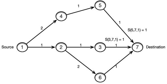
The way we solve that is by adding a new SRLG constraint to the problem which forces the path to be unique. Basically we have four binary variables which can be either 1 or 0, we make sure that they are less or equal to 3, in that way it’s never true that all the four binary variables are never true at the same time.

where $x^k_{ij}$ and $x^{k’}_{i’j’}$ are binary decision variables indicating whether links $(i, j)$ and $(i’, j’)$ are used by paths $k$ and $k’$, respectively. $S(i, j, g)$ is a binary parameter that equals 1 if link $(i, j)$ belongs to SRLG $g$, and 0 otherwise. $M$ is the set of paths ${1, 2, \ldots, K}$. $E$ is the set of links in the network.

Relevant code snippet

# Define SRLGs
srlg_data = {
    (3, 7): [1],
    (5, 7): [1]
}

# SRLG constraints
for (i, j) in srlg_data:
    for (i_prime, j_prime) in srlg_data:
        if (i, j) != (i_prime, j_prime):
            for g in set(srlg_data[(i, j)]) & set(srlg_data[(i_prime, j_prime)]):
                for k in range(K):
                    for k_prime in range(k+1, K):
                        prob += x[i, j, k] + x[i_prime, j_prime, k_prime] <= 1


Minimum total cost: 8.0
Path 1: 1 -> 4 -> 5 -> 7
Path 2: 1 -> 2 -> 6 -> 7

Weighted SRLG Algorithm

For large networks, solving the ILP problem with SRLG constraints can be difficult to solve. The Weighted Shared Risk Link Group (WSRLG) algorithm is an approach designed to address the complexity of the Integer Linear Programming (ILP) computation needed for the MIN-SUM problem with SRLG constraints in large networks. The WSRLG algorithm is a heuristic that helps to find disjoint paths by taking into account the SRLG constraints while aiming to minimize the sum of the path costs.

The core idea of WSRLG is to adjust the cost of each link in the network based on the number of SRLG groups to which the link belongs. This cost is then used in a k-shortest paths algorithm to find disjoint paths. Here’s a step-by-step breakdown of the WSRLG algorithm:

Calculate Adjusted Link Cost( $C_{comp}(i,j)$): The algorithm introduces a new composite cost for each link in the network, which is a weighted combination of the original link cost and the SRLG factor. The composite cost calculation aims to increase the cost of using links that are part of larger SRLGs, thereby discouraging their selection and reducing the risk of simultaneous failures. The composite cost, which is a combination of the original link cost and the weighted SRLG factor. The formula for $C_{comp}(i,j)$ is:

where $d_{ij}$ is the original cost of the link, $d_{ij}^{max}$ is the maximum link cost in the network, $SRLG(i,j)$ is the number of SRLGs to which link (i,j) belongs, $SRLG^{max}$ is the maximum number of SRLGs that any link belongs to, and $\alpha$ is a weight factor for SRLG. By adjusting $\alpha$, the algorithm can be tuned to emphasize either cost efficiency or SRLG-disjointness.

Weight Factor ($\alpha$): The weight factor $\alpha$ is a crucial part of the cost calculation as it balances the importance of the link’s original cost against the risk posed by SRLG membership. By adjusting $\alpha$, the algorithm can be tuned to emphasize either cost efficiency or SRLG-disjointness.

Path Cost Calculation ($C_{path}(p, q)$): The algorithm calculates the total cost of the disjoint paths from source node p to destination node q. It sums the composite costs of all the links used in each disjoint path and adds them up to find the overall cost for the set of paths.

Binary Search for $\alpha$: To find an optimal solution, a binary search is performed to find the best value of $\alpha$. The algorithm iteratively adjusts $\alpha$ to find the lowest possible $C_{path}(p, q)$ that still results in at least K disjoint paths, where K is the required number of disjoint paths. The binary search terminates when the change in $\alpha$ is less than a small value $\epsilon$, indicating that the optimal value has been closely approximated.

Implement k-Shortest Paths Algorithm with SRLG Constraints: The modified k-shortest paths algorithm is then used to find the disjoint paths. It starts by finding the first shortest path using the adjusted link costs. The links (and associated nodes) that are part of this path are then removed from consideration for subsequent paths to ensure disjointedness.

Iterative Search: The algorithm proceeds iteratively to find additional paths by repeating the process with the remaining links and nodes, recalculating the k-shortest paths each time to find the next disjoint path.

Determine Number of Disjoint Paths ($K(p,q)$): After each iteration of finding a disjoint path, the algorithm checks if the number of paths found satisfies the required number. If not, the algorithm adjusts $\alpha$ and repeats the process.

By using this approach, WSRLG aims to find a compromise between minimizing the total cost of the paths and reducing the risk posed by SRLG-related failures. This makes the algorithm particularly useful for designing robust networks where it is crucial to consider not only the cost but also the reliability and redundancy of the paths.

For below is the pseudocode, not putting the real code to minimize the clutter and information load.

Procedure WSRLG(Graph G, Node source, Node destination, Integer K, Dictionary srlg_data, Float epsilon)

    Function compute_srlg(Node i, Node j)
        Return length of srlg_data[(i, j)] + length of srlg_data[(j, i)]

    Function compute_cost(Node i, Node j, Float alpha)
        srlg_count <- compute_srlg(i, j)
        Return (1 - alpha) * (original_costs[(i, j)] / max_cost) + alpha * (srlg_count / max_srlg)

    original_costs <- dictionary with edge (i, j) as keys and G[i][j]['weight'] as values
    max_cost <- maximum value of original_costs
    max_srlg <- maximum of compute_srlg for each edge in G

    Function find_disjoint_paths(Float alpha)
        H <- copy of Graph G
        costs <- dictionary with edge (i, j) as keys and compute_cost(i, j, alpha) as values
        Assign costs to edge attribute 'cost' in H

        disjoint_paths <- empty list

        For k from 0 to K - 1
            Try
                path <- shortest_path in H from source to destination using 'cost' as weight
                Append path to disjoint_paths
                Remove intermediate nodes from path in H to ensure node disjointness
                For each edge (i, j) in path
                    For each srlg in srlg_data values
                        If (i, j) in srlg or (j, i) in srlg
                            For each edge in srlg
                                If edge exists in H
                                    Remove edge from H
            Except NetworkXNoPath
                Break from the loop

        Return disjoint_paths

    min_alpha <- 0
    max_alpha <- 1
    optimal_alpha <- None

    While max_alpha - min_alpha > epsilon
        alpha <- (min_alpha + max_alpha) / 2
        disjoint_paths <- find_disjoint_paths(alpha)

        If length of disjoint_paths equals K
            optimal_alpha <- alpha
            Break from the loop
        Else If length of disjoint_paths is less than K
            max_alpha <- alpha
        Else
            min_alpha <- alpha

    If optimal_alpha is None
        optimal_alpha <- min_alpha

    Return find_disjoint_paths(optimal_alpha)

End Procedure

References

• Linear Programming and Algorithms for Communication Networks
• Suurballe’s algorithm