Introduction

One of the things I have been trying to play recently with is Discrete Event Simulation(DES). I think it is a powerful tool for validating ideas. In this post, we will look at a toy epidemic model to simulate SIS/SIR models.

In Epidemic modeling, there are two classic models - SIS and SIR models. The models divide the population into different categories corresponding to different stages of the epidemic.

1. Susceptible(S): Susceptible individuals can contract the disease.
2. Infected(I): Infected individuals have already been contracted the disease.
3. Recovered(R): Recovered individuals are recovered from the disease and can not be infected again.

SIS Model

In case of SIS, the main assumption is that an infected person can get infected again after recovering. The state transition diagram looks like:

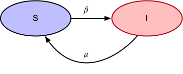
• $\beta$ is the probability of transitioning from Susceptible(S) to Infected(I)
• $\mu$ is the probability of transitioning from Infected(I) to Susceptible(S)

SIR Model

In case of SIR, the main assumption is that an infected person can not get infected again. The state transition diagram looks like:

• $\beta$ is the probability of transitioning from Susceptible(S) to Infected(I)
• $\mu$ is the probability of transitioning from Infected(I) to Recovered(R)

SIS Simulation

We will have a generic Simulation class to help model both models, which takes state transition functions as an argument and handles various state transitions as the simulation run.

Generate the Initial Graph

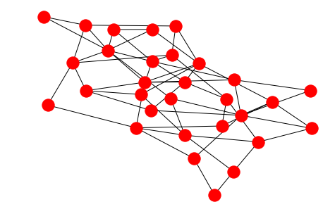
Here is a random graph of 30 Nodes and 60 edges.

import matplotlib.pyplot as plt
import networkx as nx
import random
import simulation as sm

G = nx.gnm_random_graph(30, 60)
pos=nx.layout.spring_layout(G)
nx.draw(G, pos=pos)

Initial State and State Transition Functions

Initial state function creates a dictionary of nodes with initial state set to S for all nodes and one random node is set to state I. The function returns a dictionary which will be passed to Simulation class to set that as an attribute to all the nodes.

def initial_state(G):
    state = {}
    for node in G.nodes:
        state[node] = 'S'
    
    patient_zero = random.choice(list(G.nodes))
    state[patient_zero] = 'I'
    return state

State Transition function assumes probability of 10% for both $\beta$ and $\mu$.

MU = 0.1
BETA = 0.1

def state_transition(G, current_state):
    next_state = {}
    for node in G.nodes:
        if current_state[node] == 'I':
            if random.random() < MU:
                next_state[node] = 'S'
        else: # current_state[node] == 'S'
            for neighbor in G.neighbors(node):
                if current_state[neighbor] == 'I':
                    if random.random() < BETA:
                        next_state[node] = 'I'

    return next_state

Then we pass both functions and initialize our simulation

sim = sm.Simulation(G, initial_state, state_transition, name='SIS model')

Initial state

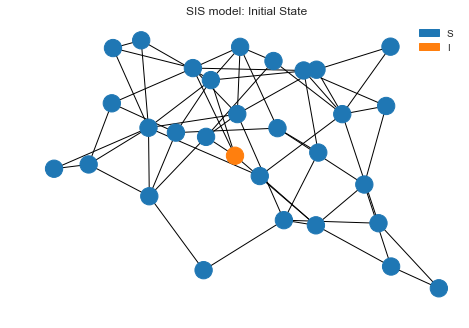
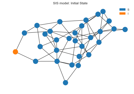
Let’s draw the initial state before we kick of the simulation. We can see one node is infected and everyone else is in S state.

sim.draw()

Simulation Run and Plot

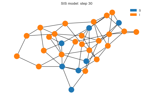
Now let’s run the simulation for 30 steps and see what’s the final state looks like after that.

sim.run(30)
sim.draw()

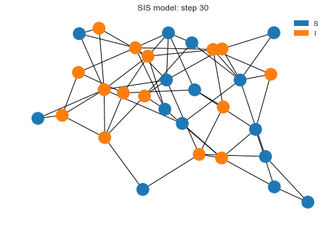
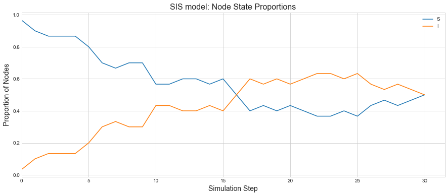
We can see we have lot more nodes infected but not every node is infected. If we plot the states, we can see how both states transitioned. It seems like after 16 steps, system is running into a somewhat steady state.

sim.plot()

What if we change the infection probability to be a bit higher.

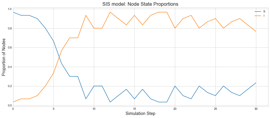
Let’s increase the $\beta$ probability to be 40% this time. So more people should be infected more and less people will be coming into a S state.

MU = 0.1
BETA = 0.40

sim = sm.Simulation(G, initial_state, state_transition, name='SIS model')
sim.draw()

After 30 steps, we have lot more nodes infected.

sim.run(30)
sim.draw()

We can see that proportions of Infected nodes rise quickly and the system is staying that way as people are getting more infected than the rate of recovery.

sim.plot()

SIR Simulation

The initial parts of graph initialization etc. will remain the same. So we will skip those steps.

Initial State and State Transition Functions

The initial state function will remain the same. The main difference will be in the state transition function. If a node is Infected, then it will transition to Recovered Sate with probability $\mu$ rather than transitioning back to Susceptible(S) state.

def state_transition(G, current_state):
    MU = 0.1
    BETA = 0.1
    next_state = {}
    for node in G.nodes:
        if current_state[node] == 'I':
            if random.random() < MU:
                next_state[node] = 'R'
        elif current_state[node] == 'S':
            for neighbor in G.neighbors(node):
                if current_state[neighbor] == 'I':
                    if random.random() < BETA:
                        next_state[node] = 'I'

    return next_state

Initializing the simulation.

sim = sm.Simulation(G, initial_state, state_transition, name='SIR model')

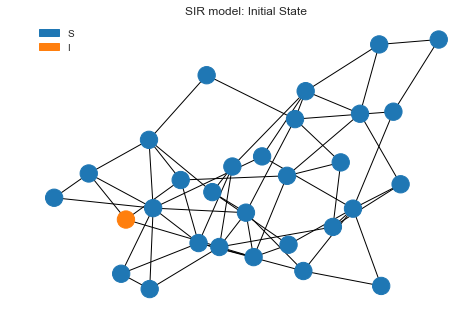
Initial state

Let’s draw the initial state before we kick of the simulation. We can see one node is infected and everyone else is in S state.

sim.draw()

Simulation Run and Plot

Now let’s run the simulation for 30 steps and see what’s the final state looks like after that.

sim.run(30)
sim.draw()

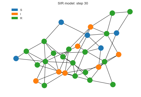
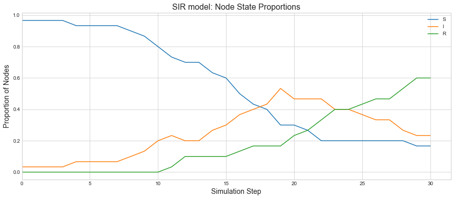
We can see as the recovered state goes high, infections are coming low as that proportion of population is not getting infected anymore.

sim.plot()

Conclusion

In this blog, we looked at few simple toy models simulating SIS/SIR epidemic models. The main idea was to showcase the power of Discrete Event Simulation(DES) for validating ideas. In future, we will use this for modeling certain network related problems.

References

• A First Course in Network Science
• Compartmental models in epidemiology