Motivation

Following up from our previous post on Bayesian Finite Mixture Models, here are my notes on Non-Finite mixture model.

Non-finite Mixture Models

Bayesian finite mixture models can be used when we have a prior knowledge or some good guess on the number of groups present in the dataset. But if we do not know this beforehand, then we can use Non-Finite mixture models. Bayesian solution for this kind of problems is related to Dirichlet process.

Dirichlet Process(DP)

We briefly mentioned about Dirichlet distribution in the previous post Bayesian Finite Mixture Models, which is a generalization of beta distribution, similarly Dirichlet Process is an infinite-dimensional generalization of Dirichlet distribution. The Dirichlet distribution is a probability distribution on the space of probabilities, while Dirichlet Process is a probability distribution on the space of distributions. A Dirichlet Process is a distribution over distributions. When I first read this, my mind went
.

What this means is, that a single draw from a Dirichlet distribution will give us a probability and a single draw from a Dirichlet Process will give us a Dirichlet distribution. For finite mixture models, we used Dirichlet distribution to assign a prior for the fixed number of clusters, A Dirichlet Process is a way to assign a prior distribution to a non-fixed number of clusters.

Some properties of Dirichlet Process(DP)

Let G be a Dirichlet Process distributed: $ G \sim DP (\alpha, G_{0}) $

Where $ G_{0} $ is the base distribution and $ \alpha $ is the positive scaling parameter.

• A DP is specified by a base distribution H and a positive real number $ \alpha $ called the concentration or scaling parameter.
• $G_{0}$ is the expected value of DP, this means that DP will generate distributions around the base distribution. An analogous way to think about is the mean of a Gaussian distribution.
• As $ \alpha $ increases, the realizations becomes less and less concentrated.
• In the limit $ \alpha \rightarrow \infty $, the realizations from DP will be equal to the base distribution.

Stick Breaking Process

One way to view DP is the so-called stick breaking process. Imagine, that we have a stick of length 1, then we break that stick into two parts (does not have to be equal), we keep one part aside and keep breaking the other part again and again. In practice, we limit this breaking process to some predefined value K. Other parameter which plays a role in the stick breaking process is $ \alpha $. As we increase the value of $ \alpha $, stick is broken into smaller and smaller parts. At $ \alpha \rightarrow 0 $, we don’t break the stick and at $ \alpha \rightarrow \infty $, we break the stick into infinite parts.

for some visual aid, check this blog out Bayesian non-parametric.

Example

We will go back to our example used in Bayesian Finite Mixture Models, and this time we will not define the number of clusters explicitly.

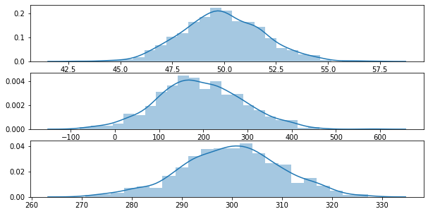
Let’s generate 3 random Gaussian distributions and mix them together.

import arviz as az
import matplotlib.pyplot as plt
import pandas as pd
import pymc3 as pm
import scipy.stats as stats
import seaborn as sns

data_size = 1000
y0 = stats.norm(loc=50, scale=2).rvs(data_size)
y1 = stats.norm(loc=200, scale=100).rvs(data_size)
y2 = stats.norm(loc=300, scale=10).rvs(data_size)
y_data = y0 + y1 + y2
y_data = pd.Series(y_data)
fig, ax = plt.subplots(3,1, figsize=(10,5))
sns.distplot(g0, ax=ax[0])
sns.distplot(g1, ax=ax[1])
sns.distplot(g2, ax=ax[2])

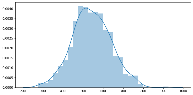
fig, ax = plt.subplots(figsize=(10,5))
sns.distplot(y_data)

Let’s use the stick breaking process where we are limiting the number of clusters to K.

N = len(y_data)
K = 20

def stick_breaking(alpha):
    beta = pm.Beta("beta", 1., alpha, shape=K)
    w = beta * pm.math.concatenate([[1.],
    tt.extra_ops.cumprod(1. - beta)[:-1]])
    return w

with pm.Model() as model_q4:
    alpha = pm.Gamma("alpha", 1., 1.)
    w = pm.Deterministic('w', stick_breaking(alpha))
    
    means = pm.Normal('means', mu=y_data.mean(), sd=10, shape=K)
    sd = pm.HalfNormal('sd', sd=100, shape=K)

    y_pred = pm.NormalMixture("y_pred", w, means, sd=sd, observed=y_data)
    
    trace_q4 = pm.sample(1000, tune=3000, nuts_kwargs={'target_accept': 0.9})

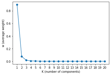
Let’s plot the Weights vs K Components, We can see that after K=3, the weights becomes flat. This tells us that the number of clusters in the data are around 3.

xs = np.arange(K)
ys = trace_q4["w"].mean(axis=0)
plt.plot(xs, ys, marker="o")
plt.xticks(xs, xs+1)
plt.xlabel("K (number of components)")
plt.ylabel("w (average weight)")
_ = plt.show()

References

Bayesian Analysis with Python
Bayesian Non-Parametrics