Motivation

I have been lately looking at Bayesian Modelling which allows me to approach modelling problems from another perspective, especially when it comes to building Hierarchical Models. I think it will also be useful to approach a problem both via Frequentist and Bayesian to see how the models perform. Notes are from Bayesian Analysis with Python which I highly recommend as a starting book for learning applied Bayesian.

Mixture Models

In statistics, mixture modelling is a common approach for model building. A Model built by simpler distributions to obtain a more complex model. For instance,

• Combination of two Gaussian’s to describe a bimodal distribution.
• Many Guassian’s to describe any arbitrary distributions.

We can use a mixture of models for modelling sub-populations or complicated distributions which can not be modelled with simpler distributions.

Finite Mixture Models

In Finite mixture models, as the name suggests, we mix a known number of models together with some weights associated for each model. Probability density of the observed data is a weighted sum of the probability density for K subgroups of the data where K is the number of models.

Here, \(w_{i}\) is the weight for each group and all the weights should sum to 1. The components \(p_{i}(y_{i}|\theta_{i})\) can be anything like Guassian, Poisson all the way to neural networks. We should know the number of K in advance, this can be either we know it beforehand or need to provide educated guess.

Categorical Distribution

Similar to our use of Bernoulli distribution to model two outcomes (0 or 1), we can use Categorical distribution to model K outcomes.

Dirichlet distribution

Dirichlet distribution is a generalization of the beta distribution. We use Beta distribution for two outcomes, one with probability p and the other 1-p. Beta distribution returns a two element vector like (p,1-p). If we want to extend beta distribution to three outcomes, we can use vector like (p,q,r). For K outcomes, we use a vector \(\alpha\) with length K. Check this post out for more intuitive detailsVisualizing Dirichlet Distributions

How to choose K

One of the main concerns with finite mixture models is how to decide the number of K. Generally one tries with a lower number of K and increase it gradually after evaluating model. In Bayesian modelling, we use evaluate models using posterior-predictive checks like WAIC or LOO.

Example

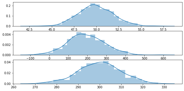
Let’s take a look at an example by first generating 3 random Gaussian distributions

import arviz as az
import matplotlib.pyplot as plt
import numpy as np
import operator
import pandas as pd
import pymc3 as pm
import scipy.stats as stats
import seaborn as sns

data_size = 1000
y0 = stats.norm(loc=50, scale=2).rvs(data_size)
y1 = stats.norm(loc=200, scale=100).rvs(data_size)
y2 = stats.norm(loc=300, scale=10).rvs(data_size)
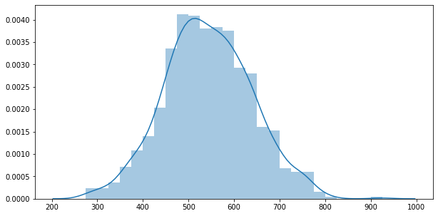
y_data = y0 + y1 + y2
y_data = pd.Series(y_data)
fig, ax = plt.subplots(3,1, figsize=(10,5))
sns.distplot(g0, ax=ax[0])
sns.distplot(g1, ax=ax[1])
sns.distplot(g2, ax=ax[2])

fig, ax = plt.subplots(figsize=(10,5))
sns.distplot(y_data)

Let’s try with clusters 2,3 and 4

clusters = [2, 3, 4]
models = []
traces = []
for cluster in clusters:
    with pm.Model() as model:
        p = pm.Dirichlet('p', a=np.ones(cluster))
        means = pm.Normal('means',
                          mu=y.mean(),
                          sd=10, shape=cluster)
        sd = pm.HalfNormal('sd', sd=100)
        y = pm.NormalMixture('y', w=p, mu=means, sd=sd, observed=y_data)
        trace = pm.sample()
        traces.append(trace)
        models.append(model)

Comparing the WAIC and LOO scores, we can see that the lowest score is for 3 Clusters.

cmp_df = az.compare({
    "2_clusters": traces[0],
    "3_clusters": traces[1],
    "4_clusters": traces[2]
}, ic="waic")
cmp_df

cmp_df = az.compare({
    "2_clusters": traces[0],
    "3_clusters": traces[1],
    "4_clusters": traces[2]
}, ic="loo")
cmp_df

Next

In next post, we will look into Non-Finite Mixture models.

References

Bayesian Analysis with Python
Visualizaing Dirchilet Distribution