It is almost impossible for someone coming from a purely mathematical background with little exposure to applications to understand how to go about formulating a real-world problem in mathematical terms. - Dantzig.

In our previous post, we explored the Min. Max Link Utilization problem using Linear Programming. The focus was on optimizing network traffic distribution to achieve optimal link utilization. However, this approach did not consider the potential impact on path lengths, allowing flows to be placed on longer paths without constraints. We mentioned this briefly in a passing statement. However, I thought it would be worth exploring the extended problem formulation that introduces an additional constraint to strike a balance between minimizing link utilization and controlling the deviation of paths from their shortest counterparts.

The core objective remains the same—to minimize the maximum link utilization across the network. However, we now introduce a conflicting constraint that aims to limit the extent to which paths can deviate from their shortest routes. This constraint is crucial for keeping path lengths within an acceptable range, as excessively long paths can degrade the user experience.

Mathematically, we are faced with two opposing constraints. On the one hand, we strive to minimize link utilization, which encourages the distribution of flows across multiple paths, potentially utilizing longer routes to balance the load. On the other hand, we want to restrict the path lengths to a certain threshold of their shortest counterparts, ensuring that the chosen paths stay within the optimal routes in terms of latency.

Recap

We had demands from sea, lax, ord, den, atl all sending $20 \text{Gbps}$ to iad.

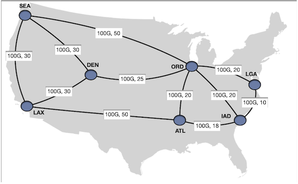
With the demands placed on the shortest paths, results in a max. link utilization of ord -> iad to 60%.

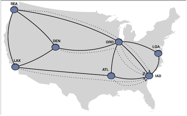
After solving for Min. max utilization, we reduced the maximum link utilization from 60% to ~33%at the expense of moving the flows to non-shortest paths. The way it was accomplished by splitting den -> iad $20 \text{Gbps}$ flow between 6.6 Gbps on den -> ord -> iad and $\text{13.3 Gbps}$ den -> ord -> lga -> iad . For atl -> iad, $20 \text{Gbps}$ flow was split between $\text{6.6 Gbps}$ atl -> ord -> iad and $\text{13.3 Gbps}$ on atl -> iad.

Maximum link utilization: 0.33%

Demand from sea to iad:
sea -> ord -> lga -> iad: 20.0

Demand from lax to iad:
lax -> atl -> iad:        20.0

Demand from ord to iad:
ord -> iad:               20.0

Demand from den to iad:
den -> ord -> lga -> iad: 13.3
den -> ord -> iad:        6.6

Demand from atl to iad:
atl -> ord -> iad:        6.6
atl -> iad:               13.3

For atl to iad, the shortest path cost is 18. We kept most of the flow on the shortest path and moved ~30% of traffic to a longer path with a cost of 40, an increase of ~122%.

For den to iad, the shortest path cost is 45. We kept ~30% (6.6Gbps) on the shortest path and moved ~70% of the traffic to a longer path with a cost of 55, which is an increase of ~22%. The IGP Cost represents latency, so the higher the IGP cost, the higher the latency.

So clearly, the latency inflation from atl to iad is much higher, more than doubled, which may be undesirable. For den to iad, ~70% of our traffic moved away from the non-shortest path; that could be also undesirable. So the question is can we do better without compromising too much on our original goal of minimizing the maximum link utilization.

Path Cost Constraints to Limit Latency Inflation

To limit the total cost of carrying a flow along a path to remain within a certain threshold, it is necessary to introduce some path cost constraint. However, putting a plain constraint that the sum of the path cost should be less than some value and looking for solutions that fit the constraint may not be feasible. This is because paths are not explicitly defined entities in how LP problems are formulated. Instead, flows are typically represented through variables associated with edges. The pattern of these flow variables across the network implicitly determines the decision of which path a flow takes.

One alternative is to find like K shortest paths, then use binary variables to indicate whether a particular path is chosen for a flow. However, this formulation of problems increases the number of variables and constraints, especially for large networks with many possible paths. So instead, what we will do is add the following constraint $sum(flow[f,i,j] \times cost[i,j]) \le (X \times \text{shortestPathCost} \times \text{demand[a,b]})$. The reason to have demand[a,b], the amount of demand between the source and destination pair on the right-hand side, is to make sure both left and right-hand side comparisons are done on a similar scale.

We can express this constraint as follows:

For each flow f:
    sum(flow[f, i, j] * cost[i, j] for each edge (i, j)) <= (1+X) * shortest_path_cost[f] * demand of f

Here, flow[f, i, j] represents the amount of flow f carried on edge (i, j), cost[i, j] represents the cost of traversing edge (i, j), and shortest_path_cost[f] represents the cost of the shortest path for flow f. Relevant code additions to our problem definition:

# Calculate the shortest path cost for each demand
for src, tgt, _ in demands:
    shortest_path_cost = nx.shortest_path_length(G, source=src, target=tgt, weight='cost')
    shortest_path_costs[(src, tgt)] = shortest_path_cost

#Path cost constraint
for src, tgt, amt in demands:
    prob += lpSum(flow_vars[src, tgt, i, j] * G[i][j][0]['cost'] for i, j in G.edges()) <= 1.2 * amt * shortest_path_costs[(src, tgt)] 

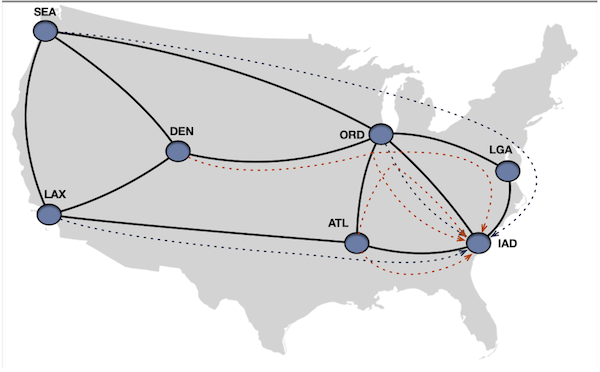
Solving the problem through the LP solver, we get the following result:

Maximum link utilization: 0.33%

Demand from sea to iad:
sea -> ord -> lga -> iad :       20.0 (Cost 80. At lga->iad flow merges.)
sea -> den -> ord -> lga -> iad: 20.0 (Cost 85. At lga->iad flow merges.)

Demand from lax to iad:
lax -> atl -> iad:               13.3 (Cost 68)
lax -> den -> ord -> iad:        6.6  (Cost 75)

Demand from ord to iad:
ord -> iad:                      20.0 (Cost 20)

Demand from den to iad:
den -> ord -> lga -> iad:       13.3 (Cost 55)
den -> ord -> iad:              6.6  (Cost 45)

Demand from atl to iad:
atl -> iad:                     20.0 (Cost 20)

After analyzing the results, we found that the solver successfully maintained a maximum link utilization rate of 33%. This was achieved by having the lga -> iad link carry 20+13.3 = 33.3 Gbps of traffic. However, this time, the demand from atl to iad was kept on the shortest path while the exact maximum link utilization was maintained by splitting the demands sea -> iad and lax -> iad. The latency deviation from the shortest path was kept under the 20% constraint.

The path from den to iad remained unchanged, but the longest path for that demand had a 22% higher latency than the shortest path, which is just slightly over our constraint. The problem would have been unfeasible if the constraint was not met, but this was not the case here. Our constraint is represented as amount of flow × edge cost ≤ 1.2 × 20(shortest path cost) × 45 (demand). The left-hand side evaluates to 13.3 × 55, which satisfies the constraint (731.5 < 1080).

The main idea is that the constraint considers the path cost and the amount of flow carried by each edge. The product of the flow amount and the edge cost allows for flexibility in flow allocation. Adjusting the flow distribution enables the solver to satisfy the constraint while accommodating paths with slightly higher latencies.

However, there is one thing I would like to change about the solution. The 70% of the flow for den to iad is on the longer latency path. It would be better if most of the demand was on shorter paths and the spillovers were on the longer route. Let’s introduce slack variables and see if they can help here. But before that, let’s take a detour and cover some fundamentals.

A Quick LP Solver Primer

Some of the iterative methods which Linear optimization solvers could use are simplex method, an active set method, or interior point method. They work by computing a sequence of progressively better solutions until an exact optimal solution is found or a satisfactory solution within acceptable tolerances in floating-point numbers is found. Although these methods employ different approaches, their goal is the same - to find the best possible solution.

Simplex Method

The simplex method was invented by George Dantzig in 1947. This method uses the corner points of the feasible region as its iterates. At each iteration, the algorithm chooses a neighboring corner point in a way that improves or does not change the objective value. When the algorithm can no longer improve the objective value, it terminates with the current corner point as an optimal solution.

Anecdote about George Dantzig

George Dantzig, an American mathematician and statistician, was born in Portland, Oregon. He is widely known as the “father of linear programming.” There is a famous anecdote about him that goes like this: When he was a graduate student, he arrived late to a statistics class and saw two unsolved problems written on the board. He mistook them for homework assignments, solved them, and turned them in. Later, he found out that the problems were long-standing and unsolved statistical problems.

Coming back to Simplex, let’s look at an example. Here is a list of constraints and our goal is to find the maximum value of y which satisfies the constraint.

Here is a visual representation of the constraints with the feasible region shaded in blue.

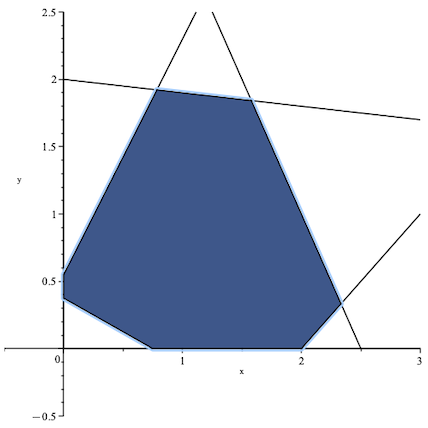
To find the optimal solution, the first step is to identify the feasible point with the highest y value using a simplex-based method. This method begins by constructing an initial feasible point or corner point. For example, let’s assume that the initial point is (0.75, 0).

The simplex-based method evaluates neighboring corner points in relation to the current point, determining which point offers the most improvement to the objective function. If the current point’s objective function is better than all its neighboring corner points, the algorithm stops, and the current point is considered optimal. However, if a neighboring point results in the highest improvement of the objective function, even if it does not change the value, then the current point is updated to this point, and the process repeats.

In this particular example, the algorithm evaluates three new points before reaching the optimal solution. The plot below illustrates the sequence of points evaluated by the algorithm.

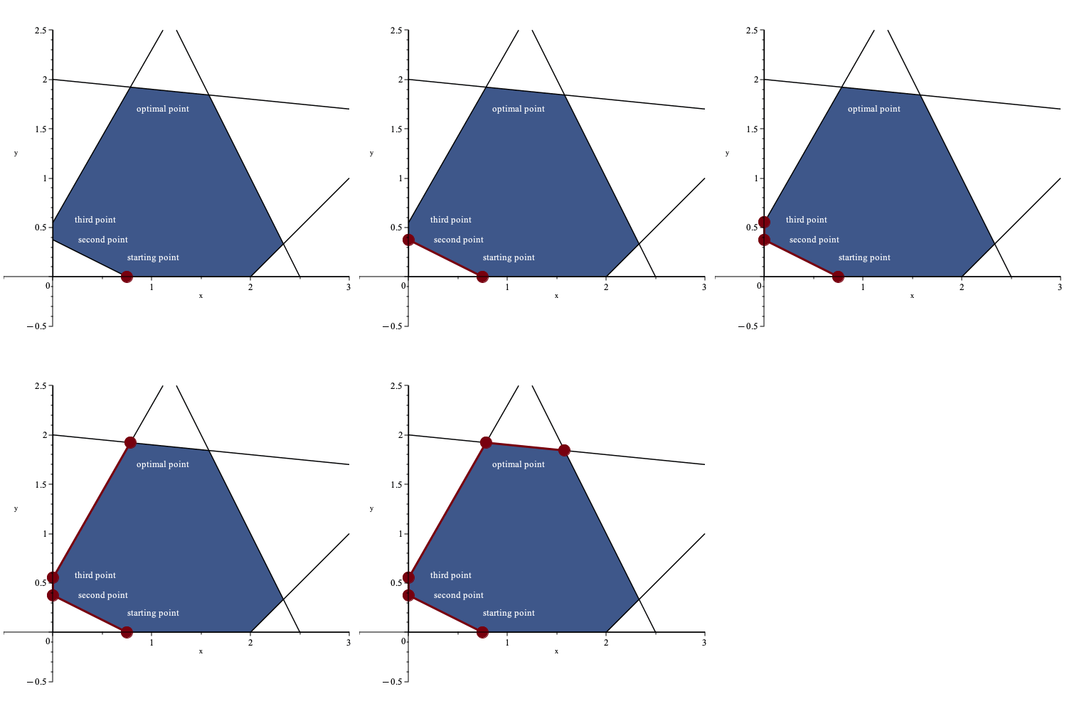
In this scenario, there was only one possible solution because the objective function was maximized at a single point within the feasible region. However, this is not always the case. If the objective function is parallel to one of the edges of the feasible region, there can be infinitely many solutions.

To explain this better, let’s consider the same feasible region as before, but with a new objective function. Suppose our new objective function is to maximize $0.1x + y$. In the graph, the green line represents the contour of the objective function in its maximized state. The two red points indicate the corner points that are optimal solutions to the maximization problem, and every point on the green line between these two points is also optimal.

If you use a simplex-based method to solve the problem, you will get one of the two corner points as the solution.

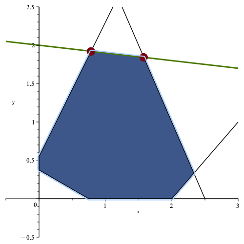
In higher dimensions, there are three possible ways for the contour of the objective function to intersect the feasible region. It can intersect the feasible region at a single point, along an edge (which leads to infinite optimal solutions), or along a face of the polytope (which also leads to infinite optimal solutions). If any of these cases occur, a simplex-based method will always be able to find a corner point as an optimal solution, provided one exists.

Active Set Method

In case of active set method, In each iteration, the algorithm identifies a subset of constraints known as the active set. The active set is a representation of the constraints that are active for the problem at an optimal solution.

To compute a new point x’, the algorithm adds a step direction Δx to the current point x in each iteration. The new point x’ that is obtained satisfies the current active set with equality. The aim is to optimize the change in the objective value from x to x’.

Moreover, the active set is adjusted until the algorithm identifies the active set for an optimal solution. If the number of constraints is greater than the number of variables in a linear optimization problem, the active set method will consider active sets of size equal to the number of variables.

Interior Point Method

In an interior point method, each iteration considers points that are strictly within the feasible region except for the initial point, which may be outside the feasible region.

In each iteration, a new point x’ is computed from the current point x by finding a step direction Δx. The step direction is chosen to optimize the change in objective value from x to x’. The parameter α is used to ensure that the new point x’ lies strictly within the feasible region.

For instance, suppose we use the same feasible region and the same objective function as the simplex method example above. In that case, the iterates of an interior point method might look similar to the plot below. Here, the initial point is infeasible.

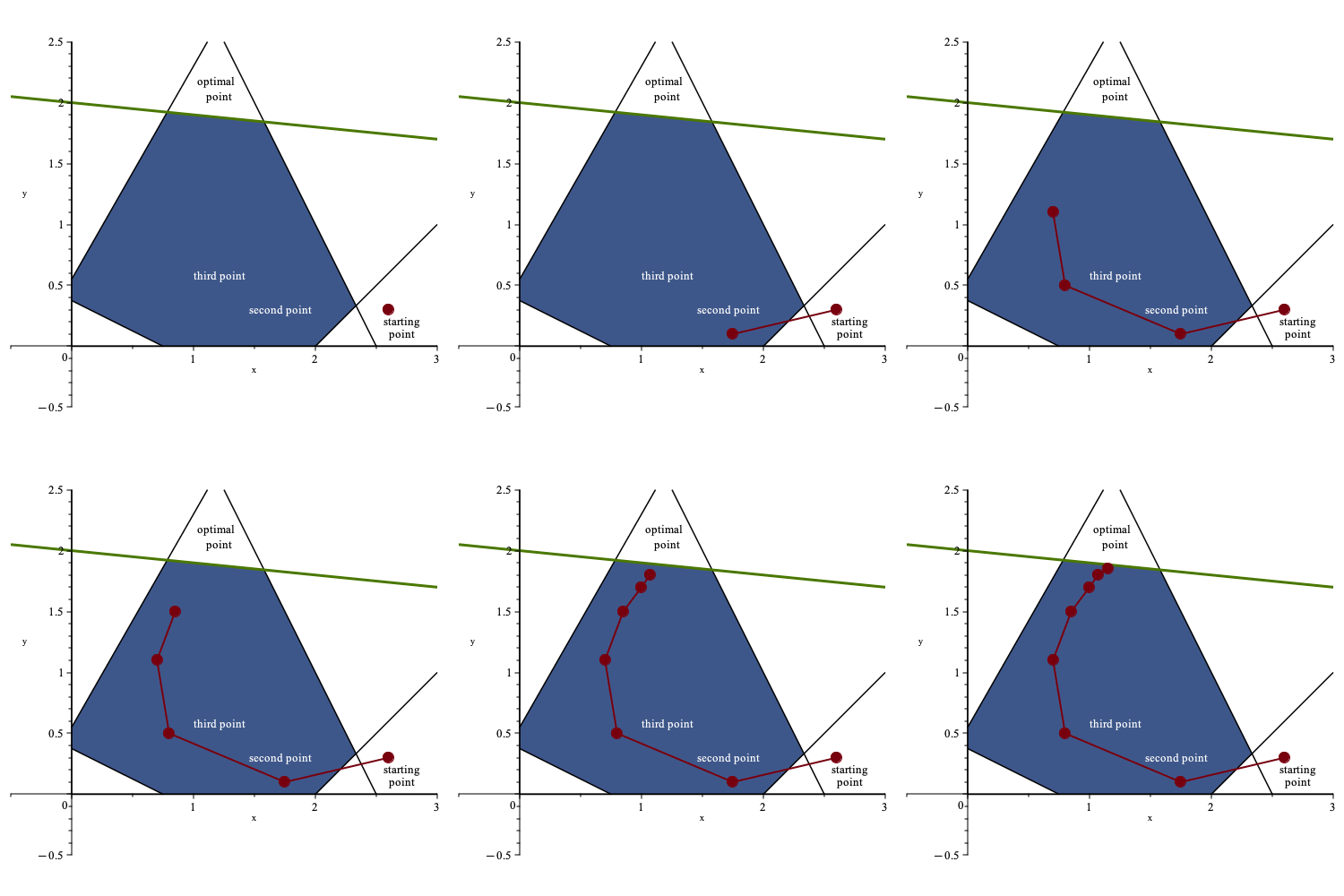
In this problem, the interior point method doesn’t identify a corner point as its solution. Instead, it finds a point that lies in the middle of the optimal solutions lines. This behavior is common with interior point methods. Although in this simple example, an interior point method may take more iterations than a simplex-based method since there are only a few corner points that can be visited. However, in larger problems with higher dimensions, the number of iterations for an interior point method can be much smaller than a simplex-based method.

Slack Variables

Slack variables play a vital role in linear programming as they enable the conversion of inequality constraints into equality constraints. This conversion is crucial in using the Simplex algorithm. Slack variables are used to measure the difference between the left and right sides of an inequality and indicate the amount of “slack” or “leeway” available to meet the constraint precisely.

Introduction of Slack Variables

Slack variables are additional variables introduced to convert inequality constraints into equality constraints. They represent the difference between the left-hand side and the right-hand side of an inequality constraint. Slack variables help solve LP problems by measuring the slack in the constraints. Let’s consider a few examples to understand slack variables better:

Example 1: Non-negative Slack Variable Suppose you have the following constraint in a linear programming problem:

Introduce a non-negative slack variable to convert this inequality constraint into an equality constraint; let’s call it s. The constraint becomes:

The slack variable s represents the difference between the left-hand side $x + y$ and the right-hand side 10. If $x + y \lt 10$, the slack variable s will take a positive value to equal the constraint. If $x + y = 10$, the slack variable s will be zero.

Example 2: Non-positive Slack Variable Now, let’s consider another constraint:

In this case, you introduce a non-positive slack variable, often called a surplus variable; let’s denote it as s’. The constraint becomes:

The surplus variable s' represents the difference between the left-hand side $x + y$ and the right-hand side 10. If $x + y \gt 10$, the surplus variable s' will take a positive value to equal the constraint. If $x + y = 10$, the surplus variable s' will be zero.

Example 3: Equality Constraint If you have an equality constraint, such as:

In this case, no slack or surplus variable is needed because the constraint is already an equality.

Positive and Negative Slack Variables

Slack variables are typically non-negative because they represent the slack or the amount by which an inequality constraint is satisfied. However, in some cases, like the one I am going to introduce negative slack variables.

Negative slack variables can arise when dealing with constraints in the form of “greater than or equal to” inequalities. In such cases, the slack variable is subtracted from the left-hand side of the constraint to convert it into an equality.

For example, consider the constraint:

By introducing a negative slack variable s, the constraint becomes:

Here, the negative slack variable s represents the amount by which the left-hand side $x + y$ exceeds the right-hand side 10. If $x + y \gt 10$, the negative slack variable s will take a positive value to equal the constraint.

The interpretation of positive and negative slack variables is as follows:

• Positive slack variable: It represents the unused or excess resources in a “less than or equal to” constraint. It indicates how much the constraint is satisfied or underutilized.
• Negative slack variable: It represents the excess or surplus in a “greater than or equal to” constraint. It indicates how much the constraint is exceeded or over utilized.

Here is a visual representation of a simple two-dimensional problem for Slack Constraint

• Constraint 1: $2x + y \leq 10$
• Constraint 2: $x + 2y \leq 8$

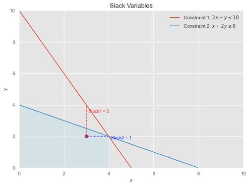
The blue-shaded area shows the feasible region, where all the constraints are satisfied. The red dot represents a sample point (3, 2) within the feasible region.

The dashed red line represents the slack variable for the constraint $2x + y \leq 10$. It indicates the vertical distance between the example point and the constraint line. In this case, the slack variable for Constraint 1 is 2, which means that there is an unused capacity of 2 units in Constraint 1 at the example point.

On the other hand, the dashed blue line represents the slack variable for the constraint $x + 2y \leq 8$. It shows the horizontal distance between the example point and the constraint line. In this case, the slack variable for Constraint 2 is 1, indicating an unused capacity of 1 unit in Constraint 2 at the example point.

Adding Slack To Our Problem

let’s define some notation first. For each demand $d=(s_{d},t_{d},A_{d})$ and each node $n \in V$,

• $s_{d}$ is the source node of demand $d$.
• $t_{d}$ is the target (destination) node of demand $d$.
• $A_{d}$ is the amount of demand (flow) that needs to be routed from $s_{d}$ to $t_{d}$.

$C_{shortest,s_{d},t_{d}}$ is the shortest path cost between source and destination node. $S_{s_{d},t_{d}}$ is the slack variable representing slack for a given demand.

We can move the $S_{s_{d},t_{d}}$ on the left hand and that is a familiar notation we saw earlier.

Modified Objective Function:

We modify the object function from just minimizing the max utilization, we also add slack variable in the objective function with a penalty factor, which kind of provides a variation scale on how much the solver should give a weight the slack variable.

The relevant code modification looks like this.

# Slack Variables
slacks = LpVariable.dicts("Slack", [(src, tgt) for src, tgt, _ in demands], 0, None)  # Slack variables

P = 1  # Penalty factor for using slack variables
prob += max_util + lpSum([P * slacks[src, tgt] for src, tgt in slacks]), 
"Minimized max_util with slack penalty"

#Path cost constraint
for src, tgt, amt in demands:
    prob += lpSum(flow_vars[src, tgt, i, j] * G[i][j][0]['cost'] for i, j in G.edges() 
                  if "dmd" not in i and "dmd" not in j) <= 1.2 * amt * shortest_path_costs[(src, tgt)] + slacks[(src, tgt)], f"Routing cost with slack for {src} to {tgt}"

The results from the solver are displayed below. The maximum link utilization remains at 33%. However, we can see a significant difference i.e. for the demands that are split, the majority of the demand is on the shortest path. This approach appears to be a better trade-off as we can keep the link utilization low while still having the majority of the flows on the shortest path.

## Normalized Output

Maximum link utilization: 0.33333333
Demand from sea to iad:
sea -> ord -> lga -> iad :      20.0 (Cost 80.At lga->iad flow merges.)
sea -> den -> ord -> lga -> iad:20.0 (Cost 85.At lga->iad flow merges.)

Demand from lax to iad:
lax -> atl -> iad:        13.3 (Cost 68)
lax -> den -> ord -> iad:  6.6 (Cost 75)

Demand from ord to iad:
ord -> iad               : 12.0 (Cost 20)
ord -> lga -> iad        :  8.0 (Cost 30)

Demand from den to iad:
den -> ord -> lga -> iad:  5.3 (Cost 55)
den -> ord -> iad:        14.6 (Cost 45)

Demand from atl to iad:
atl -> iad            :   20.0 (Cost 20)

One aspect, which I didn’t show was that although we introduced slack variables, LP Solver ultimately does not end up using them. However, formulating the problem in this way still encourages the solver to examine the solution space we are aiming for. I would be interested to hear a more detailed explanation from someone with greater familiarity in Operations Research.

Conclusion

In this post we revisited the original minimizing maximum link utilization. We improvised the problem by adding additional constraints to limit flows to be placed on paths below certain threshold of the shortest path cost. Although partially successful, the majority of split demands still used longer paths. We improvised the problem further by introducing slack variables to make sure that majority of the demands were placed on the shorter path.

References

• MMLU in Network Flow Optimization